Confidentiality in ABS business data using Pufferfish differential privacy

This paper investigates a potential use of Pufferfish differential privacy to maintain data confidentiality in ABS business data

Released
24/10/2022

Introduction

As part of the ABS’s broader strategic direction, the Data Access and Confidentiality Methodology Unit (DACMU) aims to design and implement a confidentiality method that achieves a better risk-utility trade-off subject to data and output requirements. This ensures the ABS can enhance data utility in statistical collections while providing state of the art privacy protection to data providers. Furthermore, it is important that the new confidentiality method can be generally applied to a broad range of household and business statistics publications across the ABS for consistency purposes. Under the Census and Statistics (Information Release and Access) Determination 2018, the ABS provides passive confidentiality, which protects data providers (within particular industries) who can demonstrate that the release of an ABS statistical output would likely enable their identification or accurate estimation of one or more of their attributes. These data providers are called passive claimants. This effectively puts responsibility on data providers to notify the ABS for privacy protection, subject to checking by the ABS. The work outlined in the paper investigates an instantiation of Pufferfish differential privacy (DP) through log-Laplace multiplicative perturbation to protect sugarcane production estimates sourced from an administrative dataset. If successful, this could be applied to data that the ABS collects from households and businesses, as well as statistics produced from administrative data sources. This would greatly improve the utility of the information.

The current confidentiality method for protecting passive claimants is consequential suppression; an aggregate statistic (e.g. a total) is not published if a passive claimant’s value that contributes to the statistic is sensitive. The value is then suppressed which is referred to as primary suppression. This leads to additional suppressions that are required to prevent the calculation of the primary suppressed value based on related statistics. This is referred to as consequential suppression. Suppression is an output confidentiality method which focuses on protecting aggregate outputs i.e. suppression is applied to the aggregate outputs but not to the true values of unit-level data.

Consequential suppression is no longer viable for the following reasons:
I. It limits the ABS’s capability to meet increasing user demand for more detailed statistics due to complexity in applying consequential suppression across multiple small geographic areas. There is demand for this space from the ABS Agriculture Statistics collections.
II. It restricts the ABS's ability to produce timely, flexible and user-specified outputs as geospatial differencing exposes units resulting in further suppression.
III. Research has shown that suppression is not as effective as perturbation with privacy protection.
IV. It does not help meet user demand for more detailed unit-level analysis using alternative data sources.
V. It is extremely resource intensive to apply and it needs an automated privacy approach to reduce resources required to produce ABS statistics.
VI. As the ABS moves towards increasing use of administrative datasets, direct engagement with data providers through surveys will be reduced.

Log-Laplace multiplicative perturbation improves data utility by enabling more detailed statistics to be safely published compared to suppression. This is because log-Laplace multiplicative perturbation is an input confidentiality method that perturbs a passive claimant’s unit-level value before it is used to produce aggregate statistics. This implies that the output aggregate statistics are naturally protected. Unlike suppression, additional processes are not required to protect the final statistical outputs. As a result, log-Laplace multiplicative perturbation is easier to implement than suppression, even as datasets and statistical outputs become complex. An example is publishing integrated datasets from other sources such as the Business Longitudinal Analysis Data Environment (BLADE). In addition, this approach protects against geospatial differencing risks where a passive claimant’s value may be recovered from differencing aggregate outputs from overlapping geographic regions.

Another advantage of the log-Laplace multiplicative perturbation is that it satisfies an instantiation of Pufferfish DP. Pufferfish DP is a framework for generating privacy definitions which are variations of differential privacy. These privacy definitions protect “secrets” by limiting the amount of information that users of a statistical output can learn about these “secrets” in the data. Pufferfish DP provides flexibility with the customisation of the “secrets” in a statistical collection that the ABS wants to protect. This property aligns with the ABS’s passive confidentiality policy. I.e. the sensitive variables or values of a passive claimant are the “secrets” the ABS wants to protect.

Our instantiation of Pufferfish offers a privacy protection guarantee by connecting the p% rule with the Pufferfish DP framework. The p% rule is used in the ABS and other national statistical offices to determine if a passive claimant’s value requires privacy protection. The p% rule is defined as follows: if a passive claimant’s value can be estimated to within p% of its reported value, then it requires protection. In our instantiation, the “secrets” are statements that take a form of “passive claimant A’s reported value is within p% of the value y”. Log-Laplace multiplicative perturbation protects these “secrets” by ensuring users of our statistical outputs cannot confidently determine a passive claimant’s sensitive value to within p% of its reported value, unless a user was already quite confident before observing the statistical outputs.

We have chosen the SRA sugarcane dataset as a test case and examined the data utility loss and disclosure risk from log-Laplace multiplicative perturbation. The structure of the paper is as follows: We will first briefly discuss other confidentiality methods we have considered as part of the investigation in section 2. We then provide the mathematical proof of our Pufferfish DP instantiation which connects the p% rule in section 3. Finally, we will present the case study results in section 4.

Background

The ABS investigated two other input confidentiality methods as alternatives to suppression. They are data imputation method and removal of passive claimant units. However, we have found that log-Laplace multiplicative perturbation is more effective than these methods. The following provides a brief description of each method and its suitability for the ABS Agriculture Statistics collections.

The data imputation method replaces a passive claimant’s sensitive value with one that is imputed using values of similar records. A key step is building an appropriate model from the observed data. However, it is challenging to define a set of criteria for “similar” records because it is difficult to balance privacy and utility. The donor records will need to be similar to the passive claimants but not so similar that they could reveal sensitive information about the passive claimants. A second complication is one of practicality. Due to the sparsity of Agriculture data, particularly Agriculture Census, some passive claimants might not have donor records that are similar enough to produce a satisfactory imputed value. This means that a different set of criteria is needed for obtaining a sufficiently large pool of possible donors. An example of the data imputation method is data smearing where a passive claimant’s sensitive value is replaced with an average value calculated from the subpopulation of records which are similar to the passive claimant’s record.

Removal of passive claimant units protects passive claimants’ information by removing their records before publication estimates are calculated. The primary argument against this method is that it will result in negative bias in both cell estimates and cell counts. This method was implemented and tested with the Agriculture Census 2015-2016 publication, which highlighted some more pertinent arguments against this method. For example, all chicken production in TAS and WA are estimated as 0, nursery production in ACT is 0 and mushroom production in WA is 0. This could affect public trust in the ABS because it is public knowledge that there are chicken farms in TAS and WA but the ABS releases data suggesting otherwise. The key commodities at the national level are largely unaffected. If this method is implemented for the Agriculture Census 2020-2021 publication, it will change the economic story because all estimates will be artificially deflated compared to the previous publication. It is easy to implement methods such as log-Laplace multiplicative perturbation which is unbiased and does not suffer from this problem. In the next section, we will detail our instantiation of Pufferfish DP that incorporates the p% rule but we will first describe the general form of the DP framework.

2.1. Definition of differential privacy

The following is the mathematical definition of \(\epsilon\)-differential privacy (Dwork and Roth, 2014).

Definition (\(\epsilon\)-differential privacy): Given a privacy parameter \(\epsilon\), a (potentially randomised) algorithm M satisfies \(\epsilon\)-differential privacy if for all \(W\subseteq Range(\mathcal{M})\) and for neighbouring databases \(D\) and \(D'\) that differ in only one record (i.e. one has one more record than the other), the following holds:

\(P(\mathcal{M}(D)\in W)\le e^\epsilon P(\mathcal{D'}\in W)\tag{2.1.1}\)

The original concept of \(\epsilon\)-differential privacy aims to ensure that the presence or absence of an individual record in a microdata set does not significantly affect statistical outputs produced from the microdata. Since statistical outputs produced from an \(\epsilon\)-differential privacy method are insensitive to the presence or absence of individual records in the microdata set, differential privacy limits how much information data users can learn from the statistical outputs about any individual record. Let \(\epsilon\) denote the value controlling the upper bound of information users can gain. Variations of \(\epsilon\)-differential privacy exist with similar aims.

Desfontaines and Pejo (2020) describe the key contribution of DP as defining anonymity as a property of the process of generating confidential outputs from a dataset, rather than as a property of the dataset itself. Bambauer et. al. (2013) use several examples to demonstrate how the use of the strict DP definition in (2.1.1) can have significant impact on data utility and lead to significant errors in data analysis. There has been considerable amount of research on variants or extensions of DP and adapt these definitions to different contexts and assumption to enhance data utility while maintaining confidentiality. Desfontaines and Pejó (2020) highlight that there are approximately 200 different definitions, inspired by DP, in the last 15 years. Table 2.2 summarises seven key dimensions for describing variants or extensions of DP. According to the seven dimensions in Table 2.2, Pufferfish DP is an extension of DP that allows different definitions of neighbourhood (2) and background knowledge (4). The “neighbourhoods” are pairs of secrets in a discriminative pair and the background knowledge is the set of data evolution scenarios. Section 3.1 elaborates on this when describing Pufferfish privacy for p% intervals.

Table 2.2: The seven dimensions and their usual motivation
DimensionsDescriptions
(1) quantification of privacy losshow is the privacy loss quantified across outputs?
(2) definition of neighborhoodwhich properties are protected from the attacker?
(3) variation of privacy losscan the privacy loss vary across inputs?
(4) background informationhow much prior knowledge does the attacker have?
(5) formalism knowledge gainhow to define the attacker's knowledge gain?
(6) relative knowledge gainhow to measure relative knowledge gain?
(7) computing powerhow much computational power can the attacker use?

Source. Adapted (Desfontaines and Pejó, 2020, p.290)

Our proposed instantiation of Pufferfish differential privacy for q% intervals

Key notation:
NotationDefinition
\(q\)A parameter that controls the size of the interval that is protected by Pufferfish privacy for q% intervals (see Definition 3.1.4). To make notation cleaner in definitions, theorems and proofs, let \(q\in(0, 1)\). E.g. Pufferfish privacy for 15% intervals means \(q=0.15\).
\(p\)A parameter that controls the definition of disclosure based on the p% rule. To make notation cleaner in definitions, theorems and proofs, let \(p\in(0, 1)\). E.g. 15% rule means \(p=0.15\).
\(\mathbb{S}\)The set of potential secrets that is protected by Pufferfish privacy for q% intervals (see Definition 3.1.4).
\(\mathbb{S}_{pairs}\)The set of discriminative pairs of secrets in Pufferfish privacy for q% intervals (see Definition 3.1.4).
\(s_{i}\)The statement that record \(i\)'s true value is in some pre-specified q% interval.
\(\sigma_{[I]}\)The statement that record \(i\)'s true value is in interval \(I\).
\(\mathbb{D}\)The set of data evolution scenarios for Pufferfish privacy for q% intervals (see Definition 3.1.4). Data evolution scenarios represent assumptions about how the data was generated.
\(\theta\)A prior probability distribution in \(\mathbb{D}\).
\(\epsilon\)The privacy parameter in Pufferfish privacy for q% intervals (see Definition 3.1.4).
\(\mathcal{M}\)A perturbation mechanism for protecting privacy in data.
\(\omega\)An output of a perturbation mechanism \(\mathcal{M}\).
\(W\)The set of all possible outputs from a perturbation mechanism \(\mathcal{M}\).
\(X\)Laplace distributed random variable.
\(e^{X}\)Log-Laplace distributed random variable, where \(X\) is a Laplace distributed random variable.
\(b\)The dispersion parameter for the Laplace distributed random variable \(X\).
\(c\)Bias correction factor for the log-Laplace multiplicative perturbation mechanism.

Kifer & Machanavajjhala (2014) offered a Pufferfish DP instantiation that protects intervals formed by a multiplicative factor, and proposed a log-Laplace multiplicative perturbation mechanism that satisfies that instantiation. We prove that the log-Laplace multiplicative perturbation mechanism also protects q% intervals. In section 3.1, we will describe the definition of our Pufferfish DP instantiation for q% intervals. In section 3.2, we will provide the mathematical proof that shows log-Laplace multiplicative perturbation satisfies our instantiation of Pufferfish DP for q% intervals i.e. guarantee privacy protection based on the p% rule. Given the q% interval is larger than p% interval specified by the p% rule, we will be ensuring that a data user cannot confidently determine if a passive claimant’s true value is within p% by protecting the q% interval.

3.1. Pufferfish privacy for q% intervals

There are three essential components that form the Pufferfish DP framework,

  • A set of potential of secrets \(\mathbb{S}\)
  • A set of discriminative pairs of secrets, \(\mathbb{S}_{pairs}\subseteq\mathbb{S}\times\mathbb{S}\)
  • A collection of data evolution scenarios \(\mathbb{D}\)

The set of potential secrets is what a data custodian wants to protect in statistical outputs. In our instantiation, it takes the form of a statement such as “record \(i\)’s true value is in this q% interval”. This forms the domain for the set of discriminative pairs of secrets. The ABS wants to ensure data users cannot distinguish, in a probabilistic sense, which of statements \(s_i\) or \(s_j\) in a discriminative pair \(\left(s_i, s_j\right)\) is true. For example, consider the discriminative pair (record \(i\)’s true value lies in the q% interval around \(y\), record \(i\)’s true value lies in the q% interval around \(\frac{1+q}{1-q}y\)). Note that these are adjacent q% intervals, which means they are non-overlapping but end-to-end. This choice of discriminative pair means that upon observing the statistical outputs, a data user cannot significantly improve their prior knowledge about which of two adjacent q% intervals is more likely to contain record \(i\)’s true value. The data evolution scenarios in \(\mathbb{D}\) describe a data user’s prior knowledge about the data generation process for the underlying data from which statistical outputs are produced.

Kifer & Machanavajjhala (2014) introduced an instantiation of Pufferfish DP to offer privacy protection for intervals of the form \(\left[\alpha y, \frac{y}{a}\right)\) where \(y>0\) and \(\alpha\in\left(0, 1\right)\). For brevity, we call this the “interval around \(y\) formed by factor \(\alpha\)” hereafter. This is done by adding multiplicative perturbation noise from a log-Laplace distribution to a record’s value. Using the Pufferfish DP framework definition, we define our instantiation of Pufferfish DP for the p% privacy rule as follows,

Choose a fixed \(q\in\left(0, 1\right)\). Define the set of secrets as,

\(\mathbb{S}=\left\{\sigma_{\left[\left(1-q\right)y,\ \left(1+q\right)y\right)}:y>0\ \right\}\cup\left\{\sigma_{\left(\left(1+q\right)y,\ \left(1-q\right)y\right]}∶y<0\right\}\tag{3.1.1}\)

where \(\sigma_{\left[\left(1-q\right)y,\ \left(1+q\right)y\right)}\) is the statement that a record’s value is in the interval \(\left[\left(1-q\right)y,\ \left(1+q\right)y\right)\) and \(\sigma_{\left(\left(1+q\right)y,\ \left(1-q\right)y\right]}\) is the statement that a record’s value is in the interval \(\left(\left(1+q\right)y,\ \left(1-q\right)y\right]\).

Define the set of discriminative pairs as,

\(\mathbb{S}_{pairs}=\left\{\left(\sigma_{\left[\left(1-q\right)y,\ \left(1+q\right)y\right)},\ \sigma_{\left[\left(1+q\right)y,\frac{\left(1+q\right)^2}{1-q}y\right)}\right)∶y>0\right\}\\ \cup \left\{\left(\sigma_{\left(\frac{\left(1+q\right)^2}{1-q}y,\ \left(1+q\right)y\right]},\ \sigma_{\left(\left(1+q\right)y,\ \left(1-q\right)y\right]}\right)∶y<0\right\}\tag{3.1.2}\)

Define the set of data evolution scenarios \(\mathbb{D}\) as the set of probability distributions where

\(\theta\in\mathbb{D}\ \text{if and only if } P\left(y>0\middle|\theta\right)+P\left(y<0\middle|\theta\right)=1\tag{3.1.3}\)

That is, \(\mathbb{D}\) is the set of probability distributions with support that is contained in \(\mathbb{R}-\left\{0\right\}\)\(\theta\) is a specific probability distribution that corresponds to a data user’s prior knowledge about the data generation process.

Definition 3.1.4 (Pufferfish privacy for q% intervals): Given the set of potential secrets \(\mathbb{S}\) in (3.1.1), the set of discriminative pairs \(\mathbb{S}_{pairs}\) in (3.1.2), the set of data evolution scenarios \(\mathbb{D}\) in (3.1.3), and privacy parameter \(\epsilon>0\), a (potentially randomised) algorithm \(\mathcal{M}\) satisfies \(\left(\mathbb{S},\ \mathbb{S}_{pairs},\ \mathbb{D},\ \epsilon\right)\)-Pufferfish if

(i) for all possible outputs \(\omega\in range\left(\mathcal{M}\right)\),
(ii) for all pairs \(\left(s_i, s_j\right)\in\mathbb{S}_{pairs}\) of potential secrets,
(iii) for all distributions \(\theta\in\mathbb{D}\) for which \(P\left(s_i\middle|\theta\right)\neq0\) and \(P\left(s_j\middle|\theta\right)\neq0\),

the following holds:

\(P\left(\mathcal{M}\left(Data\right)=\omega\middle| s_i,\ \theta\right)\le e^\epsilon P\left(\mathcal{M}\left(Data\right)=\omega\middle| s_j,\ \theta\right)\tag{3.1.5}\)

\(P\left(\mathcal{M}\left(Data\right)=\omega\middle| s_j,\ \theta\right)\le e^\epsilon P\left(\mathcal{M}\left(Data\right)=\omega\middle| s_i,\ \theta\right)\tag{3.1.6}\)

Remark: (i) in definition 3.1.4 implies that the output of \(\mathcal{M}\) is discrete because if it was continuous, (3.1.5) and (3.1.6) would be trivially satisfied since \(P\left(\mathcal{M}\left(Data\right)=\omega\middle|\ldots\right)=0\) for all \(\omega\in range\left(\mathcal{M}\right)\). It is more sensible/general to write (i) for all possible sets \(W\subseteq range\left(\mathcal{M}\right)\)’ and rewrite (3.1.5) and (3.1.6) with \(P\left(\mathcal{M}\left(Data\right)\in W\middle|\ldots\right)\) instead of \(P\left(\mathcal{M}\left(Data\right)=\omega\middle|\ldots\right)\). However, we leave definition 3.1.4 as it is because Kifer & Machanavajjhala used this convention and the change would have insignificant impact on this section. For example, the proof of theorem 3.2.2 in section 3.2 would just have an outer integral \(\int_{\omega\in W}{\ldots d\omega}\) but nothing else in the proof would be adversely affected.

3.2. Proof: log-Laplace multiplicative perturbation satisfies Pufferfish differential privacy for q% intervals

We first introduce a lemma that describes the relative positions of adjacent q% intervals and adjacent intervals formed by factor \(1-q\) (\(\alpha=1-q\) in our case). We visualise their relative positions below. The square and round brackets lie on a real number line but we omit the number line to reduce clutter. The diagrams merely show that adjacent intervals formed by factor \(1-q\) contain adjacent q% intervals, a fact which we prove in Lemma 3.2.1.

Adjacent intervals formed by factor \(1-q\):

\(\left[\ \ \ \ \ \ \ \ \ \ \ \ \ \ \ \ \ \ \ \ \ \ \ \ \ \ \ \ \ \ \ \ \ \ \ \ \ \ \ \ \ \ \ \ \ \ \ \ \ \ \ \ \ \ \ \ \ \ \ \ \ \ \ \ \ \ \ \ \ \ \ \ \ \ \ \ \ \ \ \ \ \ \ \ \ \right)\left[\ \ \ \ \ \ \ \ \ \ \ \ \ \ \ \ \ \ \ \ \ \ \ \ \ \ \ \ \ \ \ \ \ \ \ \ \ \ \ \ \ \ \ \ \ \ \ \ \ \ \ \ \ \ \ \ \ \ \ \ \ \ \ \ \ \ \ \ \ \ \ \ \ \ \ \ \ \ \ \ \ \ \ \ \ \right)\)

\(\left(1-q\right)y\ \ \ \ \ \ \ \ \ \ \ \ \ \ \ \ \ \ \ \ \ \ \ \ \ \ \ \ \ \ \ \ \ \ \ \ \ \ \ \ \ \ \ \ \ \ \ \ \ \ \ \ \ \ \ \ \ \ \ \ \ \ \ \ \ \ \ \ \ \ \frac{y}{1-q}\ \ \ \ \ \ \ \ \ \ \ \ \ \ \ \ \ \ \ \ \ \ \ \ \ \ \ \ \ \ \ \ \ \ \ \ \ \ \ \ \ \ \ \ \ \ \ \ \ \ \ \ \ \ \ \ \ \ \ \ \ \ \ \ \ \ \ \ \ \ \ \ \ \ \ \ \ \ \ \frac{y}{\left(1-q\right)^3}\)

Adjacent q% intervals:

\(\left[\ \ \ \ \ \ \ \ \ \ \ \ \ \ \ \ \ \ \ \ \ \ \ \ \ \ \ \ \ \ \ \ \ \ \ \ \ \ \ \ \ \ \ \ \ \ \ \ \ \ \ \ \ \ \ \ \ \ \ \ \ \ \ \ \ \ \ \ \ \ \right)\left[\ \ \ \ \ \ \ \ \ \ \ \ \ \ \ \ \ \ \ \ \ \ \ \ \ \ \ \ \ \ \ \ \ \ \ \ \ \ \ \ \ \ \ \ \ \ \ \ \ \ \ \ \ \ \ \ \ \ \ \ \ \ \ \ \ \ \ \ \ \ \right)\)

\(\left(1-q\right)y\ \ \ \ \ \ \ \ \ \ \ \ \ \ \ \ \ \ \ \ \ \ \ \ \ \ \ \ \ \ \ \ \ \ \ \ \ \ \ \ \ \ \ \ \ \ \ \ \ \ \left(1+q\right)y\ \ \ \ \ \ \ \ \ \ \ \ \ \ \ \ \ \ \ \ \ \ \ \ \ \ \ \ \ \ \ \ \ \ \ \ \ \ \ \ \ \ \ \ \ \ \ \ \ \ \ \ \ \ \ \ \ \ \ \ \frac{\left(1+q\right)^2}{\left(1-q\right)}y\)

Lemma 3.2.1: The following inequalities, which describe the relative positions of adjacent q% intervals and adjacent intervals formed by factor \(1-q\), hold for all \(q\in\left(0, 1\right)\).

\(1+q\le\frac{1}{1-q}\\ \frac{1}{1-q}\le\frac{\left(1+q\right)^2}{1-q}\\ \frac{\left(1+q\right)^2}{1-q}\le\frac{1}{\left(1-q\right)^3}\)

Proof is provided in Appendix C.

We now prove that the log-Laplace multiplicative perturbation mechanism satisfies Pufferfish privacy for q% intervals. We follow the method of proof used in Appendix H of “Pufferfish: A Framework for Mathematical Privacy Definitions” (Kifer & Machanavajjhala, 2014).

Theorem 3.2.2: Given the set of potential secrets \(\mathbb{S}\) in (3.1.1), the set of discriminative pairs \(\mathbb{S}_{pairs}\) in (3.1.2), the set of data evolution scenarios \(\mathbb{D}\) in (3.1.3), and privacy parameter \(\epsilon>0\), the log-Laplace multiplicative perturbation mechanism

\(\mathcal{M}\left(Data=y\right)=ce^Xy\tag{3.2.3}\)

satisfies \(\left(\mathbb{S},\ \mathbb{S}_{pairs},\ \mathbb{D},\ \epsilon\right)\)-Pufferfish, where \(X\) is distributed as \(Laplace\left(0,b\right)\) with \(b=-\frac{4}{\epsilon}\ln{\left(1-q\right)}\) and \(c=1-b^2\) (bias correction factor, equal to \(\frac{1}{E\left(e^X\right)}\), which can be obtained from Appendix A.2 Proposition 4). Note that \(e^X\) has a log-Laplace distribution if \(X\) has a Laplace distribution.

Proof

Let \(f\left(t\right)\) be the probability density function (pdf) of \(t\). Let \(f\left(t\in A\right)\) be the probability that \(t\) is in the set \(A\), and \(f\left(t\middle| A\right)\) be the conditional pdf of \(t\) given \(t\in A\). Assume \(support\left(f\right)\subset\left[0,\infty\right)\) (we deal with the case \(support\left(f\right)\subset\left(-\infty,0\right]\) later). Let \(\theta=f\) and assume \(f\left(t\in\left[\left(1-q\right)y,\left(1+q\right)y\right)\right)\neq0\) and \(f\left(t\in\left[\left(1+q\right)y,\frac{\left(1+q\right)^2}{1-q}y\right)\right)\neq0\). Note \(t\) is the true value of a record from the intruder’s perspective. \(t\) is random because we assume the intruder does not know what \(t\) is.

Remarks are provided throughout the derivation of the proof to improve readability.

Regarding the q% interval:

\(P\left(\mathcal{M}\left(t\right)=\omega\middle| t\in\left[\left(1-q\right)y,\ \left(1+q\right)y\right),\ \theta\right)\\ =P\left(\ln{\mathcal{M}(t)}=\ln{\omega}\middle|\ln{t}\in\left[\ln{y}-\ln{\left(\frac{1}{1-q}\right)},\ln{y}+\ln{\left(1+q\right)}\right),\ \theta\right)\\ =P\left(\ln{c}+\ln{t}+X=\ln{\omega}\middle|\ln{t}\in\left[\ln{y}-\ln{\left(\frac{1}{1-q}\right)},\ln{y}+\ln{\left(1+q\right)}\right),\ \theta\right)\\ =P\left(\ln{t}+X=\ln{\left(\frac{\omega}{c}\right)}\middle|\ln{t}\in\left[\ln{y}-\ln{\left(\frac{1}{1-q}\right)},\ln{y}+\ln{\left(1+q\right)}\right),\ \theta\right)\)

Remark: In \(\ln{t}+X\) where \(X\) is distributed as \(Laplace\left(0,b\right)\) with \(b=-\frac{4}{\epsilon}\ln{\left(1-q\right)}\)\(\ln{t}\) and \(X\) are random. The pdf of a sum of two random variables is given by convolution. The terms before \(f\) in the integrand below come from the Laplace pdf for \(X\) evaluated at \(\ln{\left(\frac{\omega}{c}\right)}-\ln{t}\).

\(P\left(\ln{t}+X=\ln{\left(\frac{\omega}{c}\right)}\middle|\ln{t}\in\left[\ln{y}-\ln{\left(\frac{1}{1-q}\right)},\ln{y}+\ln{\left(1+q\right)}\right),\ \theta\right)\)

\(=\int_{0}^{\infty}{-\frac{\epsilon}{8\ln{\left(1-q\right)}}\exp{\left(\frac{\epsilon\left|\ln{\left(\frac{\omega}{c}\right)}-\ln{t}\right|}{4\ln{\left(1-q\right)}}\right)}f\left(\ln{t}\middle|\ln{t}\in\left[\ln{y}-\ln{\left(\frac{1}{1-q}\right)},\ln{y}+\ln{\left(1+q\right)}\right),\theta\right)}dt\\ =\int_{0}^{\infty}{-\frac{\epsilon}{8\ln{\left(1-q\right)}}\exp{\left(\frac{\epsilon\left|\ln{\left(\frac{\omega}{c}\right)}-\ln{y}+\ln{y}-\ln{t}\right|}{4\ln{\left(1-q\right)}}\right)}f\left(\ln{t}\middle|\ln{t}\in\left[\ln{y}-\ln{\left(\frac{1}{1-q}\right)},\ln{y}+\ln{\left(1+q\right)}\right),\theta\right)}dt\)

Remark: Apply \(\left|a+b\right|\le\left|a\right|+\left|b\right|\) (triangle inequality) to the (negative) exponent of the Laplace density.

\(\int_{0}^{\infty}{-\frac{\epsilon}{8\ln{\left(1-q\right)}}\exp{\left(\frac{\epsilon\left|\ln{\left(\frac{\omega}{c}\right)}-\ln{y}+\ln{y}-\ln{t}\right|}{4\ln{\left(1-q\right)}}\right)}f\left(\ln{t}\middle|\ln{t}\in\left[\ln{y}-\ln{\left(\frac{1}{1-q}\right)},\ln{y}+\ln{\left(1+q\right)}\right),\theta\right)}dt\)

\(\geq\int_{0}^{\infty}{-\frac{\epsilon}{8\ln{\left(1-q\right)}}\exp{\left(\frac{\epsilon\left|\ln{\left(\frac{\omega}{c}\right)}-\ln{y}\right|}{4\ln{\left(1-q\right)}}+\frac{\epsilon\left|\ln{y}-\ln{t}\right|}{4\ln{\left(1-q\right)}}\right)}f\left(\ln{t}\middle|\ln{t}\in\left[\ln{y}-\ln{\left(\frac{1}{1-q}\right)},\ln{y}+\ln{\left(1+q\right)}\right),\theta\right)}dt\)

Remark: Now \(\left|\ln{y}-\ln{t}\right|\le\ln{\left(\frac{1}{1-q}\right)}\) because \(\ln{t}\in\left[\ln{y}-\ln{\left(\frac{1}{1-q}\right)},\ln{y}+\ln{\left(1+q\right)}\right)\subseteq\left[\ln{y}-\ln{\left(\frac{1}{1-q}\right)},\ln{y}+\ln{\left(\frac{1}{1-q}\right)}\right)\) from Lemma 3.2.1.

\(\int_{0}^{\infty}{-\frac{\epsilon}{8\ln{\left(1-q\right)}}\exp{\left(\frac{\epsilon\left|\ln{\left(\frac{\omega}{c}\right)}-\ln{y}\right|}{4\ln{\left(1-q\right)}}+\frac{\epsilon\left|\ln{y}-\ln{t}\right|}{4\ln{\left(1-q\right)}}\right)}f\left(\ln{t}\middle|\ln{t}\in\left[\ln{y}-\ln{\left(\frac{1}{1-q}\right)},\ln{y}+\ln{\left(1+q\right)}\right),\theta\right)}dt\)

\(\geq\int_{0}^{\infty}{-\frac{\epsilon}{8\ln{\left(1-q\right)}}\exp{\left(\frac{\epsilon\left|\ln{\left(\frac{\omega}{c}\right)}-\ln{y}\right|}{4\ln{\left(1-q\right)}}+\frac{\epsilon\ln{\left(\frac{1}{1-q}\right)}}{4\ln{\left(1-q\right)}}\right)}f\left(\ln{t}\middle|\ln{t}\in\left[\ln{y}-\ln{\left(\frac{1}{1-q}\right)},\ln{y}+\ln{\left(1+q\right)}\right),\theta\right)}dt\)

Remark: Only \(f\) in the integrand depends on \(t\). Since \(f\) is a density, its integral equals \(1\).

\(\int_{0}^{\infty}{-\frac{\epsilon}{8\ln{\left(1-q\right)}}\exp{\left(\frac{\epsilon\left|\ln{\left(\frac{\omega}{c}\right)}-\ln{y}\right|}{4\ln{\left(1-q\right)}}+\frac{\epsilon\ln{\left(\frac{1}{1-q}\right)}}{4\ln{\left(1-q\right)}}\right)}f\left(\ln{t}\middle|\ln{t}\in\left[\ln{y}-\ln{\left(\frac{1}{1-q}\right)},\ln{y}+\ln{\left(1+q\right)}\right),\theta\right)}dt\)

\(=-\frac{\epsilon}{8\ln{\left(1-q\right)}}\exp{\left(\frac{\epsilon\left|\ln{\left(\frac{\omega}{c}\right)}-\ln{y}\right|}{4\ln{\left(1-q\right)}}+\frac{\epsilon\ln{\left(\frac{1}{1-q}\right)}}{4\ln{\left(1-q\right)}}\right)}\)

\(=-\frac{\epsilon}{8\ln{\left(1-q\right)}}\exp{\left(\frac{\epsilon\left|\ln{\left(\frac{\omega}{c}\right)}-\ln{y}\right|}{4\ln{\left(1-q\right)}}\right)}\exp{\left(-\frac{\epsilon}{4}\right)} \;\;\;\;\;\;\;\;\;\;\;\;\;\;\;\;\;\;\;\;\;\;\;\;\;\;\;\;\;\;\;\;\;\;\;\;\;\;\;\;\;\;\;\;\;\;\;\;\;\;\;\;\;\;\;\;\;\;\;\;\;\;\;\;\;\;\;\;\;\;\;\;\;\;\;\;\;\;\;\;\;\;\;\;\;\;\;\;\;\;\;\;\;\;(3.2.4)\)

Regarding the adjacent q% interval:

\(P\left(\mathcal{M}\left(t\right)=\omega\middle| t\in\left[\left(1+q\right)y,\frac{\left(1+q\right)^2}{1-q}y\right),\ \theta\right)\\ =P\left(\ln{\mathcal{M}\left(t\right)}=\ln{\omega}\middle|\ln{t}\in\left[\ln{y}+\ln{\left(1+q\right)},\ \ln{y}+\ln{\frac{\left(1+q\right)^2}{1-q}}\right),\ \theta\right)\\ =P\left(\ln{c}+\ln{t}+X=\ln{\omega}\middle|\ln{t}\in\left[\ln{y}+\ln{\left(1+q\right)},\ln{y}+\ln{\frac{\left(1+q\right)^2}{1-q}}\right),\ \theta\right)\\ =P\left(\ln{t}+X=\ln{\left(\frac{\omega}{c}\right)}\middle|\ln{t}\in\left[\ln{y}+\ln{\left(1+q\right)},\ \ln{y}+\ln{\frac{\left(1+q\right)^2}{1-q}}\right),\ \theta\right)\)

Remark: In \(\ln{t}+X\) where \(X\) is distributed as \(Laplace\left(0,b\right)\) with \(b=-\frac{4}{\epsilon}\ln{\left(1-q\right)}\)\(\ln{t}\) and \(X\) are random. The pdf of a sum of two random variables is given by convolution. The terms before \(f\) in the integrand below come from the Laplace pdf for \(X\) evaluated at \(\ln{\left(\frac{\omega}{c}\right)}-\ln{t}\).

\(P\left(\ln{t}+X=\ln{\left(\frac{\omega}{c}\right)}\middle|\ln{t}\in\left[\ln{y}+\ln{\left(1+q\right)},\ \ln{y}+\ln{\frac{\left(1+q\right)^2}{1-q}}\right),\ \theta\right)\)

\(=\int_{0}^{\infty}{-\frac{\epsilon}{8\ln{\left(1-q\right)}}\exp{\left(\frac{\epsilon\left|\ln{\left(\frac{\omega}{c}\right)}-\ln{t}\right|}{4\ln{\left(1-q\right)}}\right)}f\left(\ln{t}\middle|\ln{t}\in\left[\ln{y}+\ln{\left(1+q\right)},\ln{y}+\ln{\frac{\left(1+q\right)^2}{1-q}}\right),\theta\right)}dt\\ =\int_{0}^{\infty}{-\frac{\epsilon}{8\ln{\left(1-q\right)}}\exp{\left(\frac{\epsilon\left|\ln{\left(\frac{\omega}{c}\right)}-\ln{y}+\ln{y}-\ln{t}\right|}{4\ln{\left(1-q\right)}}\right)}f\left(\ln{t}\middle|\ln{t}\in\left[\ln{y}+\ln{\left(1+q\right)},\ln{y}+\ln{\frac{\left(1+q\right)^2}{1-q}}\right),\theta\right)}dt\)

Remark: Apply \(\left|a+b\right|\geq\left|a\right|-\left|b\right|\) to the (negative) exponent of the Laplace density.

\(\int_{0}^{\infty}{-\frac{\epsilon}{8\ln{\left(1-q\right)}}\exp{\left(\frac{\epsilon\left|\ln{\left(\frac{\omega}{c}\right)}-\ln{y}+\ln{y}-\ln{t}\right|}{4\ln{\left(1-q\right)}}\right)}f\left(\ln{t}\middle|\ln{t}\in\left[\ln{y}+\ln{\left(1+q\right)},\ln{y}+\ln{\frac{\left(1+q\right)^2}{1-q}}\right),\theta\right)}dt\)

\(\le\int_{0}^{\infty}{-\frac{\epsilon}{8\ln{\left(1-q\right)}}\exp{\left(\frac{\epsilon\left|\ln{\left(\frac{\omega}{c}\right)}-\ln{y}\right|}{4\ln{\left(1-q\right)}}-\frac{\epsilon\left|\ln{y}-\ln{t}\right|}{4\ln{\left(1-q\right)}}\right)}f\left(\ln{t}\middle|\ln{t}\in\left[\ln{y}+\ln{\left(1+q\right)},\ln{y}+\ln{\frac{\left(1+q\right)^2}{1-q}}\right),\theta\right)}dt\)

Remark: Now \(\left|\ln{y}-\ln{t}\right|\le3\ln{\left(\frac{1}{1-q}\right)}\) because \(\ln{t}\in\left[\ln{y}+\ln{\left(1+q\right)},\ln{y}+\ln{\left(\frac{\left(1+q\right)^2}{1-q}\right)}\right) \subseteq\left[\ln{y}+\ln{\left(1-q\right)},\ln{y}+\ln{\left(\frac{1}{\left(1-q\right)^3}\right)}\right) \\=\left[\ln{y}-\ln{\left(\frac{1}{1-q}\right)},\ln{y}+3\ln{\left(\frac{1}{1-q}\right)}\right)\) 

from Lemma 3.2.1.

\(\int_{0}^{\infty}{-\frac{\epsilon}{8\ln{\left(1-q\right)}}\exp{\left(\frac{\epsilon\left|\ln{\left(\frac{\omega}{c}\right)}-\ln{y}\right|}{4\ln{\left(1-q\right)}}-\frac{\epsilon\left|\ln{y}-\ln{t}\right|}{4\ln{\left(1-q\right)}}\right)}f\left(\ln{t}\middle|\ln{t}\in\left[\ln{y}+\ln{\left(1+q\right)},\ln{y}+\ln{\frac{\left(1+q\right)^2}{1-q}}\right),\theta\right)}dt\)

\(\le\int_{0}^{\infty}{-\frac{\epsilon}{8\ln{\left(1-q\right)}}\exp{\left(\frac{\epsilon\left|\ln{\left(\frac{\omega}{c}\right)}-\ln{y}\right|}{4\ln{\left(1-q\right)}}-\frac{3\epsilon\ln{\left(\frac{1}{1-q}\right)}}{4\ln{\left(1-q\right)}}\right)}f\left(\ln{t}\middle|\ln{t}\in\left[\ln{y}+\ln{\left(1+q\right)},\ln{y}+\ln{\frac{\left(1+q\right)^2}{1-q}}\right),\theta\right)}dt\)

Remark: Only \(f\) in the integrand depends on \(t\). Since \(f\) is a density, its integral equals \(1\).

\(\int_{0}^{\infty}{-\frac{\epsilon}{8\ln{\left(1-q\right)}}\exp{\left(\frac{\epsilon\left|\ln{\left(\frac{\omega}{c}\right)}-\ln{y}\right|}{4\ln{\left(1-q\right)}}-\frac{3\epsilon\ln{\left(\frac{1}{1-q}\right)}}{4\ln{\left(1-q\right)}}\right)}f\left(\ln{t}\middle|\ln{t}\in\left[\ln{y}+\ln{\left(1+q\right)},\ln{y}+\ln{\frac{\left(1+q\right)^2}{1-q}}\right),\theta\right)}dt\)

\(=-\frac{\epsilon}{8\ln{\left(1-q\right)}}\exp{\left(\frac{\epsilon\left|\ln{\left(\frac{\omega}{c}\right)}-\ln{y}\right|}{4\ln{\left(1-q\right)}}-\frac{3\epsilon\ln{\left(\frac{1}{1-q}\right)}}{4\ln{\left(1-q\right)}}\right)}\)

\(=-\frac{\epsilon}{8\ln{\left(1-q\right)}}\exp{\left(\frac{\epsilon\left|\ln{\left(\frac{\omega}{c}\right)}-\ln{y}\right|}{4\ln{\left(1-q\right)}}\right)}\exp{\left(\frac{3\epsilon}{4}\right)} \;\;\;\;\;\;\;\;\;\;\;\;\;\;\;\;\;\;\;\;\;\;\;\;\;\;\;\;\;\;\;\;\;\;\;\;\;\;\;\;\;\;\;\;\;\;\;\;\;\;\;\;\;\;\;\;\;\;\;\;\;\;\;\;\;\;\;\;\;\;\;\;\;\;\;\;\;\;\;\;\;\;\;\;\;\;\;\;\;\;\;\;\;\;\;\;(3.2.5)\)

Compare (3.2.4) and (3.2.5).

\(RHS\ of\ \left(3.2.5\right)=e^\epsilon\times RHS\ of\ \left(3.2.4\right)\\ LHS\ of\ \left(3.2.5\right)\le e^\epsilon\times LHS\ of\ \left(3.2.4\right)\\ P\left(\mathcal{M}\left(t\right)=\omega\middle| t\in\left[\left(1+q\right)y,\frac{\left(1+q\right)^2}{1-q}y\right),\ \theta\right)\le e^\epsilon P\left(\mathcal{M}\left(t\right)=\omega\middle| t\in\left[\left(1-q\right)y,\ \left(1+q\right)y\right),\ \theta\right)\)

A similar derivation results in

\(P\left(\mathcal{M}\left(t\right)=\omega\middle| t\in\left[\left(1-q\right)y,\ \left(1+q\right)y\right),\ \theta\right)\le e^\epsilon P\left(\mathcal{M}\left(t\right)=\omega\middle| t\in\left[\left(1+q\right)y,\frac{\left(1+q\right)^2}{1-q}y\right),\ \theta\right)\)

The case where \(support\left(f\right)\subset\left(-\infty,0\right]\) is proven by virtue of symmetry: the pdf for \(ce^Xy\), where \(y<0\), is the reflection of the pdf for \(-ce^Xy\) about \(y=0\), and every pair of adjacent q% intervals in \(\mathbb{R}^{<0}\) is the reflection (about \(y=0\)) of a pair of adjacent q% intervals in \(\mathbb{R}^{>0}\). In the case where \(y<0\), we can view the mechanism as applying three transformations sequentially: given some \(y<0\), multiply \(y\) by \(-1\) (reflection), multiply the result by \(e^X\) where \(X\) is distributed as \(Laplace\left(0,b\right)\) (perturbation), multiply the result by \(​​-1\) (reflection). The first and last transformations are deterministic. Thus, the log-Laplace multiplicative perturbation mechanism applied to negative scalars satisfies Definition 3.1.4 just like for positive scalars.

Case study: agriculture statistics with sugarcane data

The mathematical proof in the previous section shows the log-Laplace multiplicative perturbation mechanism protects q% intervals. In this case study, we use the SRA sugarcane administrative data to explore the utility and risk trade-off under different privacy parameter settings. We need to consider two privacy parameters in the log-Laplace multiplicative perturbation mechanism, ϵ and q. Both of the parameters control the dispersion of the log-Laplace perturbation distribution. The privacy parameter ϵ controls the bounds on the amount of information that a potential intruder can gain about a secret from the perturbed outputs. The secrets are passive claimants’ true values that reside within the q% intervals.

4.1. Case study design

As part of the ABS privacy policy, we are required to protect a passive claimant’s value when it violates the p% rule. For the case study, we set an arbitrary threshold of 15% as the p% rule (i.e. p=0.15 means that p% rule=15%). We then consider a disclosure risk scenario where there are only three contributors in a small area from the sugarcane dataset. We assume the largest contributor is interested in estimating the second largest contributor’s true value. We set the second largest contributor to be our passive claimant.  The third contributor is small relative to the size of the first and second largest contributors. Our study tests the effectiveness of the multiplicative perturbation mechanism under this scenario with a high risk of p% rule violation. Our case study only considers perturbing a single passive claimant.

4.2. Data structure

At the time of writing this paper, the Agriculture Statistics section within the ABS Physical and Environmental Accounts Statistics Branch has developed a roadmap to optimise the use of administrative data in the production of ABS Agriculture Statistics collections. We want to show that log-Laplace multiplicative perturbation mechanism will protect individual business data when producing statistics sourced from an administrative dataset.

We currently have access to the sugarcane data from the Levy Payer Register administrative source. For the purpose of our case study, we treat the sugarcane dataset as a census. While the sugarcane data does not contain “identified” passive claimants, users are interested in sugarcane production at fine geographical levels. This provides a similar disclosure risk scenario where Agriculture Statistics section needs to protect the passive claimants’ data in small areas.  

There are 3,865 observations in the sugarcane dataset with 4 main variables. The variables are Australian Business Number (ABN), sugarcane production (tonnes), Statistical Area Level 1 (SA1) and Statistical Area Level 2 (SA2). For the purposes of this case study, areas with missing values in ABN, SA1 or SA2 were excluded from this analysis. Sugarcane production is the variable that we want to perturb for a passive claimant.

4.3. Utility loss and disclosure risk measures

We now present our empirical and analytical estimates of utility loss and disclosure risk measurement. The empirical estimates are derived by simulation given a particular data scenario. For example, the passive claimant is the second largest contributor in a dataset of 3 units and the largest contributor is interested in estimating the passive claimant’s true value. The purpose of deriving the analytical estimates is twofold. Firstly, we can compare the empirical estimates with the analytical estimates as they should align. This helps us to verify our empirical estimates. Secondly, we can produce utility loss and disclosure risk estimates under any data scenarios (regardless of which contributor the passive claimant is or which contributor is interested in estimating the passive claimant’s true value) without running separate simulations. This can be done by plotting the analytical formulas and examine the theoretical level of utility loss and disclosure risk. However, note that the analytical formulas are only applicable for perturbing one passive claimant as our case study only considers perturbing a single passive claimant. The derivation becomes more complex as we perturb more passive claimants. Therefore, simulation is a less complex option to examine the level of utility loss and disclosure risk. We will examine the effects of perturbing multiple passive claimants in our future work.

Utility loss measure assessment

There is inevitably a degree of data utility loss when perturbing the true value of the observations. We derive the empirical and analytical RSE from the log-Laplace multiplicative perturbation for a single passive claimant to measure the level of data utility loss.

Algorithm for empirical estimation of utility loss (RSE)                                                                                                (4.3.1)

Note: q = 0.1 -> q% = 10%.

Require: input unit file
Require: A set of privacy parameters: ϵ and q
Require: Number of simulation runs M
       \(\begin{align*} \mu &= 0 &&\text{Mean of Laplace distribution} \\ b &= \left(\frac{-4}{\epsilon}\right)\ln{\left(1-q\right)} &&\text{Dispersion of Laplace distribution} \\ c &= 1 - b^2 &&\text{Bias correction factor} \end{align*}\)

for m = 1,…,M  do

       \(\begin{align*} z_m &=ce^{X_m} &&X_m \sim Laplace\left(\mu,b\right),\ \\ &&&z_m \ \text{is the multiplicative perturbation factor for each simulation run m } \end{align*} \)

       if passive claimant j then do

               \(\begin{align*} {\widetilde{y}}_{j,m}=z_my_j &&y_j \ \text{is the true value of the passive claimant j} \end{align*} \) 

       end

       /* Calculate the total of the units including the perturbed value for each simulation run m */

       \(\begin{align*} {\hat{Y}}_m=\sum_{h=1,h\neq j}^{n}y_h+{\widetilde{y}}_{j,m} &&\text{n is the total number of observations} \end{align*} \)

end

/* Calculate root mean squared error */

\(\begin{align*} RMSE=\sqrt{\frac{\sum_{m=1}^{M}{{(\hat{Y}}_m-Y)}^2}{M}} &&\text{Y is the true total} \end{align*} \)

/* Calculate RSE */

\(RSE=\frac{RMSE}{Y}\)

return RSE

return A data frame\(\ \hat{D}\)  with the perturbed value of the passive claimant \({\widetilde{y}}_{j,m}\) from each simulation m and the true values of all other units.

The analytical solution of RSE is as follows,

\(RSE_{analytical}=\frac{\sqrt{Var\left(\hat{Y}\ \right)}}{Y} \)

where,

\(Var\left(\hat{Y}\right)=\sum_{h\in n}{\left(1-a_hb_h^2\right)^{2a_h}y_h^2\left[\frac{1}{1-4a_hb_h^2}-\frac{1}{\left(1-a_hb_h^2\right)^2}\right]} \)

and 

\( a_h= \begin{cases} 1, & \text{if unit h is perturbed} \\ 0, & \text{otherwise} \end{cases} \)

and

\(b_h=\left(\frac{-4}{\epsilon}\right)\ln{\left(1-q\right)} \)
The above formula is derived by assuming a total Y is estimated using the Horvitz-Thompson estimator for a probability sampling method without replacement. We modify the formula to incorporate the effect of log-Laplace multiplicative perturbation for some unit’s values \(y_h\). The Horvitz-Thompson estimator was chosen since it is the simplest estimator for calculating weighted totals and is used in ABS surveys. We assume that the sampling method and perturbation are independent in order to derive an expression for the variance of our estimate subject to sampling error and perturbation noise. Note that under the assumptions of the design-based framework for survey sample designs, the true values \(y_h\) are constant and only the sample and perturbation factors for these values are randomly determined. The expression above is for the specific case of a completely enumerated population, meaning the only source of variance is from the perturbation. This is applicable to the sugarcane dataset as we are assuming it is a census. Full details of this derivation are presented in Appendix A.

Disclosure risk measure assessment

We derive the empirical and analytical probability of p% rule violation to examine the level of disclosure risk from log-Laplace multiplicative perturbation for a single passive claimant. We assume a contributor k to the sugarcane production in a particular area is interested in estimating passive claimant j’s contribution. This can be done by subtracting unit k’s value from the total and examining if the remainder is within p% of unit j’s true value. If it is then the p% rule is violated i.e. there is disclosure. Note that this is our definition of disclosure in our case study.

Algorithm for empirical estimation of disclosure risk probability                                                   (4.3.2)

Note: This algorithm uses the output data frame \(\hat{D}\). We use p for the input p% rule parameter instead of q in this algorithm because q in algorithm (4.3.1) is the parameter that describes the q% intervals we want to protect in Pufferfish DP. p and q can take different values. It is important to keep in mind that p is the threshold that defines disclosure (p% rule violation) and q is the intervals that Pufferfish DP protects (proved in section 3). 

Require: \(\hat{D}\)  

Require: input p% rule parameter: p [p=0.15 -> p% rule =15%]

for m = 1,......,M do

       \({\hat{Y}}_m=\sum_{h=1,h\neq j}^{n}y_h+{\widetilde{y}}_{j,m}\)

       /* Subtract the true value of contributor k, \(y_k \) from \(\hat{Y}_m\)*/

       \({\ddot{Y}}_m={\hat{Y}}_m-y_k\)

       if \({\ddot{Y}}_m\in\left[y_j\left(1-p\right),y_j\left(1+p\right)\right]\) then do

           \(P_m=1\)

       end else do

           \(P_m=0\)

       end

end

\(\begin{align*} ​​​​\gamma=\frac{\sum_{m=1}^{M}P_m}{M} &&\text{Probability of p% rule violation} \end{align*}\)

return \(\gamma\)

The analytical solution of disclosure risk (the probability of a p% rule violation) is given by,

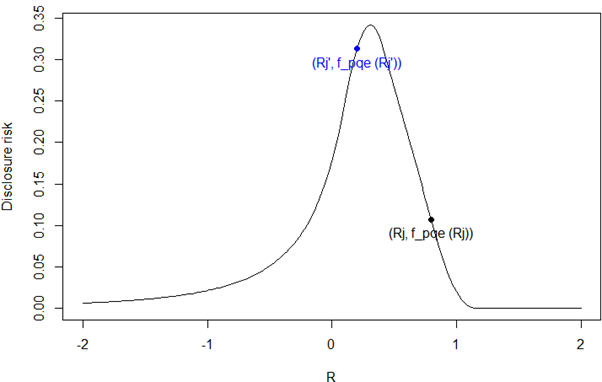
\(\begin{equation*} P\left(\left(1-p\right)y_j<\ ce^{X_j}y_j+\sum_{i=1,\ i\neq j,k}^{n}y_i<\left(1+p\right)y_j\ |\ p,b,\mu,y_1,\ldots y_n\right) \\= \begin{cases} \frac{1}{2}\left[\left(\frac{1-p-R}{c}\right)^{-\frac{1}{b}}-\left(\frac{1+p-R}{c}\right)^{-\frac{1}{b}}\right], &if \ R\le1-p-c\ \\ 1-\frac{1}{2}\left[\left(\frac{1+p-R}{c}\right)^{-\frac{1}{b}}+\left(\frac{1-p-R}{c}\right)^\frac{1}{b}\right], &if \ 1-p-c<R\le\min{\left(1-p,1+p-c\right)} \\ \frac{1}{2}\left[\left(\frac{1+p-R}{c}\right)^\frac{1}{b}-\left(\frac{1-p-R}{c}\right)^\frac{1}{b}\right], &if \ {1+p-c<R<1-p} \\ 1-\frac{1}{2}\left(\frac{1+p-R}{c}\right)^{-\frac{1}{b}}, &if \ {1-p\le R\le1+p-c} \\ \frac{1}{2}\left(\frac{1+p-R}{c}\right)^\frac{1}{b}, &if \ \max{\left(1+p-c,1-p\right)}\le R<1+p\\ 0, &if \ R\geq1+p \end{cases} \end{equation*}\)

Note that the third and fourth case cannot occur at the same time for a particular value of \(p\in(0,1)\)

where,

\(R=\frac{\sum_{h=1,\ h\neq j,k}^{n}y_h}{y_j} \)

and 

\(b=\left(\frac{-4}{\epsilon}\right)\ln{\left(1-q\right)}\)

and

\(c=1-b^2\)

The above formula is derived by assuming a data user wishes to estimate passive claimant j’s contribution \(y_j\) to some total within p% (specified by the p% rule) assuming they know contribution \(y_k\) with certainty. The formula above holds for any total containing a single passive claimant perturbed with log-Laplace multiplicative perturbation of the form \(e^{X_j}\) where \(X_j\sim Laplace(0,b)\). The result is piecewise due to the piecewise definition of the Laplace distribution and conditions on R in order for the p% interval to be valid. This formula is presented in Appendix B.1.2 Corollary (Equation b.1.3). The derivation is provided in Appendix B.1. We also derive the upper bound of disclosure risk for more than one passive claimant in Appendix B.2.

4.4. Sugarcane data case study results

We have chosen a list of ϵ and q values and perturbed the passive claimant’s value 1000 times (m=1000). We have retrieved the empirical estimates of RSE and disclosure risk probability by running algorithm (4.3.1) and (4.3.2) respectively. We have tested that 1000 replicates were sufficient to derive an adequate empirical estimate. We have also derived the analytical solution of RSE and disclosure risk. We have chosen a fixed p in algorithm (4.3.2) and vary q in algorithm (4.3.1). This is because q changes the definition of Pufferfish privacy for q% intervals through the dispersion of the Laplacian distribution (b). Therefore, we want to ensure that we have a fixed threshold for disclosure that is different from the one that defines the level of perturbation. p is set to 0.15 (p% rule = 15%) and it is our interval to define when a disclosure has occurred. It is important to keep in mind that our definition of disclosure risk is when there is a p% rule violation. So even when there is a violation, it does not mean there is disclosure because Pufferfish DP guarantees that data users cannot significantly improve their confidence in determining which q% interval a passive claimant’s true value lies within.

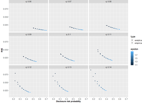
Figure 4.4.1 and 4.4.2 depict utility loss vs disclosure risk given a set of ϵ and q.  The results are within expectation as a higher RSE (utility loss) leads to a lower disclosure risk probability. This is driven by the dispersion of the Laplace distribution, b which is determined by ϵ and q and \(b=\left(\frac{-4}{\epsilon}\right)\ln{\left(1-q\right)}\).

With q fixed, a higher ϵ results in a lower b which means a lower RSE and a higher disclosure risk probability and vice versa. With a fixed ϵ, a higher q leads to a higher b which means a higher RSE and a lower disclosure risk probability and vice versa. This is consistent with what we observe in Figure 4.4.1 and 4.4.2. The graphs show some discrepancy between empirical and analytical results for small ϵ and large q. This is because b becomes large for small ϵ and large q, and that if \(b>\frac{1}{2}\), the variance of \(e^X\), where \(X_j\sim Laplace(0,b)\), is unbounded (more details presented in Appendix A.1 Proposition 2). Hence, only the empirical estimates are shown in the graphs for these particular points.

Figure 4.4.1: Utility loss (RSE) vs Disclosure risk probability, p=0.15 (p% rule=15%) (ϵ panel)

Utility loss vs Disclosure risk

Figure 4.4.1: Utility loss (RSE) vs Disclosure risk probability, p=0.15 (p% rule=15%) (ϵ panel)
Comparing utility loss and disclosure risk. Utility loss is measured by relative standard error (RSE) on the y axis and disclosure risk is measured by disclosure risk probability on the x axis. There are two types of estimates for RSE and disclosure risk probability, analytical and empirical. The graph is divided into 9 panels with each panel indicating a specific value of ϵ (ranges from 1.1 to 1.9). Within each panel, it shows the estimate of RSE and disclosure risk probability at a given ϵ and q which ranges from 0.06 to 0.14. There is an inverse relationship between RSE and disclosure risk probability, a higher RSE (utility loss) leads to a lower disclosure risk probability and vice versa.

Figure 4.4.2: Utility loss (RSE) vs Disclosure risk probability, p=0.15 (p% rule=15%) (q panel)

Utility loss vs Disclosure risk

Figure 4.4.2: Utility loss (RSE) vs Disclosure risk probability, p=0.15 (p% rule=15%) (q panel)
Comparing utility loss and disclosure risk. Utility loss is measured by relative standard error (RSE) on the y axis and disclosure risk is measured by disclosure risk probability on the x axis. There are two types of estimates for RSE and disclosure risk probability, analytical and empirical. The graph is divided into 9 panels with each panel indicating a specific value of q (ranges from 0.06 to 0.14). Within each panel, it shows the estimate of RSE and disclosure risk probability at a given q and ϵ which ranges from 1.1 to 1.9. There is an inverse relationship between RSE and disclosure risk probability, a higher RSE (utility loss) leads to a lower disclosure risk probability and vice versa.

An interesting finding is that in certain scenarios from the sugarcane dataset we tested (results not shown), perturbing a passive claimant that contributes to a particular cell potentially increases the disclosure risk of another cell that a passive claimant also contributes to. A general example is given as follows,

Passive claimant j contributes to cell A (state=QLD, Goods=sugarcane) and cell B (state=QLD, Business type=Sole Proprietor). Suppose unit j violates the p% rule in cell A but not cell B. We perturb unit j’s true value because it violates the p% rule in cell A.

   Pre-perturbation:

        Disclosure risk of unit j in cell A = 100%

        Disclosure risk of unit j in cell B = 0%
   Post-perturbation:

        Disclosure risk of unit j in cell A = 40%

        Disclosure risk of unit j in cell B = 35%

This finding means that a decrease in disclosure risk in cell A via perturbation does not always come for free as it could increase the disclosure risk of cell B. The important aspect to keep in mind is that Pufferfish DP via log-Laplace distribution offers a different type of protection than absolute protection guarantees (0 disclosure risk i.e. 0% chance of p% rule violation). Instead, Pufferfish DP guarantees that a data user cannot significantly improve their confidence in determining if the true value lies within a q% interval or an adjacent q% interval.

Conclusion

We have demonstrated that Kifer & Machanavajjhala (2014)’s Pufferfish DP instantiation offers privacy protection for our q% intervals via log-Laplace multiplicative perturbation. This means that it also offers privacy guarantees specified by the p% rule. As expected, our case study results from perturbing a single passive claimant shows that there is an inverse relationship between utility loss and disclosure risk. Pufferfish DP offers a form of privacy protection that ensures data users cannot become significantly more confident in determining if a passive claimant’s true value lies within a q% interval or an adjacent q% interval. Our case study results help us to understand the effects of different privacy parameter values on utility loss and disclosure risk. For our future work, we will utilise these results and the analytical formulas we have derived for utility loss and disclosure risk to determine an appropriate set of privacy parameters \(\epsilon\) and \(q\) for a broader suite of ABS Agriculture Statistics collections. In addition, we will assess utility loss and disclosure risk trade off from perturbing two or more passive claimants because our case study only focused on perturbing a single passive claimant. We will also consider a utility and disclosure risk assessment with unit-level data as the case study results are based on aggregated outputs. An important task ahead is that we will need to investigate some relaxed form of Pufferfish DP where the multiplicative perturbation factor is bounded. This is to avoid post-processing outputs when the mechanism introduces an extreme perturbed value, which undermines user trust in the statistics. In other words, a relaxed form of Pufferfish DP can bound the level of utility loss.

Post release changes

18/11/2022 - Relabelled mathematical definitions and equations with continuous numbering.

Bibliography

Dwork, C. and Roth, A., 2014, The Algorithmic Foundations of Differential Privacy, Foundations and Trends in Theoretical Computer Science, Vol 9, Nos. 3-4, 2014, 211-407

Kifer, D and Machanavajjhala, A., 2014: Pufferfish: A Framework for Mathematical Privacy Definition, 2014 ACM Transactions on Database Systems, Article No. 3

Desfontaines, D. and Pejó, B., 2020. Sok: Differential privacies. Proceedings on Privacy Enhancing Technologies, 2020(2), pp.288-313.

Bambauer, J., Muralidhar, K. and Sarathy, R., 2013. Fool's gold: an illustrated critique of differential privacy. Vand. J. Ent. & Tech. L., 16, p.701.

Census and Statistics (Information Release and Access) Determination 2018

Appendices - Mathematical proofs and derivations

Appendix A - Analytical formula for the variance of Horvitz-Thompson estimator

Appendix A.1 provides a general analytical formula for the variance of the Horvitz-Thompson (HT) estimator of total under simple random sampling without replacement (SRSWOR) after adjusting for perturbation of passive claimants’ values by log-Laplace multiplicative perturbation, with \(X_i \sim Laplace\left(\mu_i,b_i\right)\) for unit \(i\). A.2 incorporates bias correction into the general formula, since the expected value of a log-Laplace random variable is greater than \(1\). A.3 gives the variance formula for the case of a Census where \(\mu_i=0\). This is applicable to the Agricultural Statistics sugarcane data that we used in our case study.

A.1. Variance of HT estimator under SRSWOR

We first introduce a lemma that gives the mean of a log-Laplace distribution.

Lemma 1. If  \(X \sim Laplace\left(\mu,b\right)\), where \(b>0\), then \(E\left(e^{aX}\right)\) (moment generating function) has the following forms: ­

Case 1: If \(\left|ab\right|<1\), then

\(E\left(e^{aX}\right)=\frac{e^{a\mu}}{1-a^2b^2} \tag*{}\)

Case 2: If \(ab=-1\), then

\(E\left(e^{aX}\right)=-\frac{1}{4}e^{-\ \frac{\mu}{b}} \tag*{}\)

Case 3: If \(ab=1\), then

\(E\left(e^{aX}\right)=\frac{1}{4}e^\frac{\mu}{b} \tag*{}\)

Case 4: If \(\left|ab\right|>1\), then \(E\left(e^{aX}\right)\) is not finite.

Proof

\(E\left(e^{aX}\right)\\ =\frac{1}{2b}\int_{-\infty}^{\infty}{e^{ax}e^{-\ \frac{\left|x-\mu\right|}{b}}}dx\\ =\frac{1}{2b}\lim_{h\rightarrow\infty}{\int_{-h}^{\mu}{e^{ax}e^\frac{x-\mu}{b}}dx}+\frac{1}{2b}\lim_{h\rightarrow\infty}{\int_{\mu}^{h}{e^{ax}e^\frac{-x+\mu}{b}}dx}\\ =\frac{1}{2b}e^{-\ \frac{\mu}{b}}\lim_{h\rightarrow\infty}{\int_{-h}^{\mu}e^\frac{x\left(ab+1\right)}{b}dx}+\frac{1}{2b}e^\frac{\mu}{b}\lim_{h\rightarrow\infty}{\int_{-h}^{\mu}e^\frac{x\left(ab-1\right)}{b}dx}\\ =\frac{1}{2\left(ab+1\right)}e^{-\ \frac{\mu}{b}}\lim_{h\rightarrow\infty}{\left[e^\frac{x\left(ab+1\right)}{b}\right]_{-h}^\mu}+\frac{1}{2\left(ab-1\right)}e^\frac{\mu}{b}\lim_{h\rightarrow\infty}{\left[e^\frac{x\left(ab-1\right)}{b}\right]_\mu^h}\\ =\frac{1}{2\left(ab+1\right)}e^{-\ \frac{\mu}{b}}\lim_{h\rightarrow\infty}{\left[e^\frac{\mu\left(ab+1\right)}{b}-e^\frac{-h\left(ab+1\right)}{b}\right]}+\frac{1}{2\left(ab-1\right)}e^\frac{\mu}{b}\lim_{h\rightarrow\infty}{\left[e^\frac{h\left(ab-1\right)}{b}-e^\frac{\mu\left(ab-1\right)}{b}\right]}\)

Case 1: If \(\left|ab\right|<1\), then

\(=\frac{1}{2\left(ab+1\right)}e^{-\ \frac{\mu}{b}}e^\frac{\mu\left(ab+1\right)}{b}-\frac{1}{2\left(ab-1\right)}e^\frac{\mu}{b}e^\frac{\mu\left(ab-1\right)}{b}\\ =\frac{1}{2\left(ab+1\right)}e^{a\mu}-\frac{1}{2\left(ab-1\right)}e^{a\mu}\\ =\frac{e^{a\mu}}{1-a^2b^2}\)

Case 2: If \(ab=-1\), then

\(=-\frac{1}{4}e^{-\ \frac{\mu}{b}}\)

Case 3: If \(ab=1\), then

\(=\frac{1}{4}e^\frac{\mu}{b}\)

Case 4: If \(\left|ab\right|>1\), one of the limits is not finite so the integral for \(E\left(e^{aX}\right)\) diverges.                                                                                                                                                                                                                   ∎


Proposition 2 (True variance of HT estimator). If \({\hat{Y}}_\pi=\sum_{i\in s}{\pi_i^{-1}e^{a_iX_i}y_i}\), where \(X_i \sim Laplace\left(\mu_i,b_i\right)\), are independent, and

\(a_i = \begin{cases} 1, & \text{if unit $i$ is perturbed} \\ 0, & \text{otherwise} \\ \end{cases} \tag*{}\)

are deterministic, then the variance formula has the following forms:

Case 1: If \(a_ib_i<\frac{1}{2}\) for all \(i\), then

\(Var\left({\hat{Y}}_\pi\right)=\sum_{i\in U}{y_i^2e^{2a_i\mu_i}\left[\frac{1}{\pi_i\left(1-4a_ib_i^2\right)}-\frac{1}{\left(1-a_ib_i^2\right)^2}\right]}+\sum_{ij\in U,\ i\neq j}{y_iy_j\frac{e^{a_i\mu_i+a_j\mu_j}}{\left(1-a_ib_i^2\right)\left(1-a_jb_j^2\right)}\left(\frac{\pi_{ij}}{\pi_i\pi_j}-1\right)} \tag*{}\)

Case 2: If \(a_ib_i>\frac{1}{2}\) for some \(i\), then \(Var\left({\hat{Y}}_\pi\right)\) is not finite.

Case 3: We will not discuss the case where \(a_ib_i=\frac{1}{2}\) or \(-\frac{1}{2}\) for some \(i\) and \(a_ib_i<\frac{1}{2}\) for all other \(i\).

Proof

\(Var\left({\hat{Y}}_\pi\right)\\ =E\left({\hat{Y}}_\pi^2\right)-E\left({\hat{Y}}_\pi\right)^2\\ =E\left[\left(\sum_{i\in U}{\pi_i^{-1}\delta_ie^{a_iX_i}y_i}\right)^2\right]-E\left(\sum_{i\in U}{\pi_i^{-1}\delta_ie^{a_iX_i}y_i}\right)^2\\ =\sum_{ij\in U}{\pi_i^{-1}\pi_j^{-1}y_iy_j\boldsymbol{E\left(\delta_i\delta_je^{a_iX_i}e^{a_jX_j}\right)}}-\sum_{ij\in U}{\pi_i^{-1}\pi_j^{-1}y_iy_j\boldsymbol{E\left(\delta_ie^{a_iX_i}\right)}E\left(\delta_je^{a_jX_j}\right)}\)

(1) Consider \(\boldsymbol{E\left(\delta_i\delta_je^{a_iX_i}e^{a_jX_j}\right)}\):

\(E\left(\delta_i\delta_je^{a_iX_i}e^{a_jX_j}\right)\\ =E\left[E\left(\delta_i\delta_je^{a_iX_i}e^{a_jX_j}\middle|\delta_i\delta_j\right)\right]\\ =E\left(\delta_i\delta_je^{a_iX_i}e^{a_jX_j}\middle|\delta_i\delta_j=0\right)\Pr{\left(\delta_i\delta_j=0\right)}+E\left(\delta_i\delta_je^{a_iX_i}e^{a_jX_j}\middle|\delta_i\delta_j=1\right)\Pr{\left(\delta_i\delta_j=1\right)}\\ =E\left(0\right)\Pr{\left(\delta_i\delta_j=0\right)}+E\left(e^{a_iX_i}e^{a_jX_j}\right)\Pr{\left(\delta_i\delta_j=1\right)}\\ =E\left(e^{a_iX_i}e^{a_jX_j}\right)\Pr{\left(\delta_i\delta_j=1\right)}\)

Case 1: If \(i=j\), then we have

\(=E\left(e^{2a_iX_i}\right)\pi_i\)

From Lemma 1, if \(2a_ib_i<1\), then we have

\(=\frac{e^{2a_i\mu_i}}{1-4a_i^2b_i^2}\pi_i\\ =\frac{e^{2a_i\mu_i}}{1-4a_ib_i^2}\pi_i\)

If \(2a_ib_i>1\), then the expectation is not finite so \(Var\left({\hat{Y}}_\pi\right)\) is not finite.

Case 2: If \(i\neq j\), then we have

\(=E\left(e^{a_iX_i}\right)E\left(e^{a_jX_j}\right)\pi_{ij}\)

From Lemma 1, if \(a_ib_i<1\), then we have

\(=\frac{e^{a_i\mu_i+a_j\mu_j}}{\left(1-a_i^2b_i^2\right)\left(1-a_j^2b_j^2\right)}\pi_{ij}\\ =\frac{e^{a_i\mu_i+a_j\mu_j}}{\left(1-a_ib_i^2\right)\left(1-a_jb_j^2\right)}\pi_{ij}\)

If \(a_ib_i>1\), then the expectation is not finite so \(Var\left({\hat{Y}}_\pi\right)\) is not finite.

(2) Consider \(\boldsymbol{E\left(\delta_ie^{a_iX_i}\right)}\):

\(E\left(\delta_ie^{a_iX_i}\right)\\ =E\left[E\left(\delta_ie^{a_iX_i}\middle|\delta_i\right)\right]\\ =E\left(\delta_ie^{a_iX_i}\middle|\delta_i=0\right)\Pr{\left(\delta_i=0\right)}+E\left(\delta_ie^{a_iX_i}\middle|\delta_i=1\right)\Pr{\left(\delta_i=1\right)}\\ =E\left(0\right)\Pr{\left(\delta_i=0\right)}+E\left(e^{a_iX_i}\right)\Pr{\left(\delta_i=1\right)}\\ =E\left(e^{a_iX_i}\right)\pi_i\)

From Lemma 1, if \(a_ib_i<1\), then we have

\(=\frac{e^{a_i\mu_i}}{1-a_i^2b_i^2}\pi_i\\ =\frac{e^{a_i\mu_i}}{1-a_ib_i^2}\pi_i\)

If \(a_ib_i>1\), then the expectation is not finite so \(Var\left({\hat{Y}}_\pi\right)\) is not finite.

For the case \(2a_ib_i<1\), substitute the results from (1) and (2) into the expression for \(Var\left({\hat{Y}}_\pi\right)\). We have

\(Var\left({\hat{Y}}_\pi\right)\\ =\sum_{i\in U}{\pi_i^{-2}y_i^2\frac{e^{2a_i\mu_i}}{1-4a_ib_i^2}\pi_i}+\sum_{ij\in U,\ i\neq j}{\pi_i^{-1}\pi_j^{-1}y_iy_j\frac{e^{a_i\mu_i+a_j\mu_j}}{\left(1-a_ib_i^2\right)\left(1-a_jb_j^2\right)}\pi_{ij}}\\ -\sum_{ij\in U}{\pi_i^{-1}\pi_j^{-1}y_iy_j\frac{e^{a_i\mu_i}}{1-a_ib_i^2}\pi_i\frac{e^{a_j\mu_j}}{1-a_jb_j^2}\pi_j}\\ =\sum_{i\in U}{\pi_i^{-1}y_i^2\frac{e^{2a_i\mu_i}}{1-4a_ib_i^2}}+\sum_{ij\in U,\ i\neq j}{\pi_i^{-1}\pi_j^{-1}y_iy_j\frac{e^{a_i\mu_i+a_j\mu_j}}{\left(1-a_ib_i^2\right)\left(1-a_jb_j^2\right)}\pi_{ij}}\\ -\sum_{i\in U}{y_i^2\frac{e^{2a_i\mu_i}}{\left(1-a_ib_i^2\right)^2}}-\sum_{ij\in U,\ i\neq j}{y_iy_j\frac{e^{a_i\mu_i+a_j\mu_j}}{\left(1-a_ib_i^2\right)\left(1-a_jb_j^2\right)}}\\ =\sum_{i\in U}{y_i^2e^{2a_i\mu_i}\left[\frac{1}{\pi_i\left(1-4a_ib_i^2\right)}-\frac{1}{\left(1-a_ib_i^2\right)^2}\right]}+\sum_{ij\in U,\ i\neq j}{y_iy_j\frac{e^{a_i\mu_i+a_j\mu_j}}{\left(1-a_ib_i^2\right)\left(1-a_jb_j^2\right)}\left(\frac{\pi_{ij}}{\pi_i\pi_j}-1\right)}\)

Remark. If \(a_i=0\) for all \(i\) (i.e. no units are perturbed), the variance formula in Proposition 2 simplifies to the variance formula for the unperturbed HT estimator.

Corollary 3. If there exists a unit in the sample that is perturbed multiplicatively using log-Laplace noise with parameter \(b_i>\frac{1}{2}\), then \(Var\left({\hat{Y}}_\pi\right)\) is not finite.

Proof

The variance formula in Proposition 2 is not finite if there exists an \(i\) such that \(a_ib_i>\frac{1}{2}\), where \(a_i\) only attains values \(0\) or \(1\).

A.2. Variance with bias correction

Due to perturbation, \({\hat{Y}}_\pi=\sum_{i\in s}{\pi_i^{-1}e^{a_iX_i}y_i}\) is a biased estimator of \(Y=\sum_{i\in U} y_i\). We correct this bias by introducing a bias correction factor \(w_i\) for unit i \(i\).

Proposition 4 (Bias correction factor). \({\hat{Y}}_\pi=\sum_{i\in s}{w_i\pi_i^{-1}e^{a_iX_i}y_i} \) is an unbiased estimator of \(Y=\sum_{i\in U} y_i\) if and only if \(w_i=\left(\frac{1-a_ib_i^2}{e^{a_i\mu_i}}\right)^{a_i}\).

Proof

\({\hat{Y}}_\pi\) is an unbiased estimator of \(Y\) if and only if:

\(E\left({\hat{Y}}_\pi\right)=Y\\ E\left(\sum_{i\in s}{w_i\pi_i^{-1}e^{a_iX_i}y_i}\right)=\sum_{i\in U} y_i\)

\(E\left(\sum_{i\in U}{\delta_iw_i\pi_i^{-1}e^{a_iX_i}y_i}\right)=\sum_{i\in U} y_i\) where \(\delta_i\) is an indicator for whether unit \(i\) is in sample \(s\)

\(\sum_{i\in U}{w_i\pi_i^{-1}y_iE\left(\delta_ie^{a_iX_i}\right)}=\sum_{i\in U} y_i\\ \sum_{i\in U}{y_i\left[w_i\pi_i^{-1}E\left(\delta_ie^{a_iX_i}\right)-1\right]}=0\)

The above is true for all \(y_i\in\mathbb{R}\) if and only if \(w_i\pi_i^{-1}E\left(\delta_ie^{a_iX_i}\right)-1=0\) for all \(i\in U\). For all \(i\):

\(w_i=\frac{\pi_i}{E\left(\delta_ie^{a_iX_i}\right)}\)

Case 1: If \(a_i=0\) (i.e. unit \(i\) is not perturbed), we have

\(w_i=\frac{\pi_i}{E\left(\delta_i\right)}=\frac{\pi_i}{\pi_i}=1\)

Case 2: If \(a_i=1\) (i.e. unit \(i\) is perturbed), we have

\(w_i=\frac{\pi_i}{E\left[E\left(\delta_ie^{a_iX_i}\middle|\delta_i\right)\right]}=\frac{\pi_i}{E\left(0\right)\Pr{\left(\delta_i=0\right)}+E\left(e^{a_iX_i}\right)\Pr{\left(\delta_i=1\right)}}=\frac{\pi_i}{E\left(e^{a_iX_i}\right)\pi_i}=\frac{1}{E\left(e^{a_iX_i}\right)}\)

From Lemma 1, if \(\left|a_ib_i\right|<1\), we then have

\(w_i=\frac{1-a_ib_i^2}{e^{a_i\mu_i}}\)

Cases 1 and 2 can be combined by writing \(w_i=\left(\frac{1-a_ib_i^2}{e^{a_i\mu_i}}\right)^{a_i}\).                                                                                                                                                                                                                                                                     ∎

Corollary 5 (True variance of HT estimator with bias correction). If \({\hat{Y}}_\pi=\sum_{i\in s}{\pi_i^{-1}e^{a_iX_i}\left(\frac{1-a_ib_i^2}{e^{a_i\mu_i}}\right)^{a_i}y_i}\) where \(X_i \sim Laplace\left(\mu_i,b_i\right)\), are independent, and

\(a_i = \begin{cases} 1, & \text{if unit $i$ is perturbed} \\ 0, & \text{otherwise} \\ \end{cases} \tag*{}\)

are deterministic, then the variance formula has the following forms:

Case 1: If \(a_ib_i<\frac{1}{2}\) for all \(i\), then

\(Var\left({\hat{Y}}_\pi\right)=\sum_{i\in U}{\left(\frac{1-a_ib_i^2}{e^{a_i\mu_i}}\right)^{2a_i}y_i^2e^{2a_i\mu_i}\left[\frac{1}{\pi_i\left(1-4a_ib_i^2\right)}-\frac{1}{\left(1-a_ib_i^2\right)^2}\right]}\\ +\sum_{ij\in U,\ i\neq j}{\left(\frac{1-a_ib_i^2}{e^{a_i\mu_i}}\right)^{a_i}\left(\frac{1-a_jb_j^2}{e^{a_j\mu_j}}\right)^{a_j}y_iy_j\frac{e^{a_i\mu_i+a_j\mu_j}}{\left(1-a_ib_i^2\right)\left(1-a_jb_j^2\right)}\left(\frac{\pi_{ij}}{\pi_i\pi_j}-1\right)} \tag*{}\)

Case 2: If \(a_ib_i>\frac{1}{2}\) for some \(i\), then \(Var\left({\hat{Y}}_\pi\right)\) is not finite.

Case 3: We will not discuss the case where \(a_ib_i=\frac{1}{2}\) or \(-\frac{1}{2}\) for some \(i\) and \(a_ib_i<\frac{1}{2}\) for all other \(i\).

Proof

Since the bias correction factors \(w_i\) are deterministic, we obtain the true variance of the HT estimator after bias correction by replacing \(y_i\) with \(w_iy_i=\left(\frac{1-a_ib_i^2}{e^{a_i\mu_i}}\right)^{a_i}y_i\) in Proposition 2.

A.3. (Agriculture statistics) Variance for a census

Substitute \(\mu_i=0\)\(\pi_i=1\) and \(\pi_{ij}=1\) for all \(i,\ j\in U\) into the formula in Corollary 5. The variance formula is:

Case 1: If \(a_ib_i<\frac{1}{2}\) for all \(i\), then

\(Var\left({\hat{Y}}_\pi\right)=\sum_{i\in U}{\left(1-a_ib_i^2\right)^{2a_i}y_i^2\left[\frac{1}{1-4a_ib_i^2}-\frac{1}{\left(1-a_ib_i^2\right)^2}\right]} \tag*{}\)

Case 2: If \(a_ib_i>\frac{1}{2}\) for some \(i\), then \(Var\left({\hat{Y}}_\pi\right)\) is not finite.

Case 3: We will not discuss the case where \(a_ib_i=\frac{1}{2}\) or \(-\frac{1}{2}\) for some \(i\) and \(a_ib_i<\frac{1}{2}\) for all other \(i\).

Appendix B - Analytical derivation of disclosure risk

Appendix B.1 provides the analytical derivation of disclosure risk for a single passive claimant from log-Laplace multiplicative perturbation. Appendix B.2 derives the upper bound of disclosure risk for multiple passive claimants. We define \(p\) as the p% interval for determining if a disclosure has occurred and \(q\) as the parameter that controls the dispersion parameter of the Laplace distribution in the formula \( b=-\frac{4}{\epsilon}\ln{\left(1-q\right)}\). Note that \(p\) or \(q\)=0.3 means that p%=30%.

B.1 Derivation of disclosure risk for a single passive claimant

For the total of a quantity with n contributors, we define the true, unperturbed total as

\(Y=\sum_{i=1}^{n}y_i \tag*{}\)

where \(y_i\) represents the value of interest from contributor \(i\). We assume a scenario where contributor \(k\) is attempting to find the value of contributor \(j\) in a total where any single contributor \(j \ne k\) is a passive claimant perturbed with log-Laplace multiplicative perturbation. Assuming the perturbation is bias-corrected, the correction is defined as \(c=\frac{1-b^2}{e^\mu}\) where \(b\in(0,\frac{1}{2}\ )\) is the dispersion parameter of the log-Laplace distribution (Appendix A.2 Proposition 4). The published total will therefore have the form,

\(\hat{Y}=ce^{X_j}y_j+\sum_{i=1,\ i\neq j}^{n}y_i \tag*{}\)

where \(X_j \sim Laplace(\mu,b)\). If contributor \(k\) uses their value to attempt to learn contributor \(j\)’s value, the new total has the form,

\(\hat{Y}-y_k=ce^{X_j}y_j+\sum_{i=1,\ i\neq j,k}^{n}y_i \tag*{}\)

To assess disclosure risk according to the p% rule, we define \(p\in(0,1)\) and test if \(\hat{Y}-y_k\) falls within p% of \(y_j\). The probability of this occurring can be formally be expressed as,

\(P\left(\left(1-p\right)y_j<\ ce^{X_j}y_j+\sum_{i=1,\ i\neq j,k}^{n}y_i\ <\left(1+p\right)y_j\ |\ p,b,\mu,y_1,\ldots,\ y_n\right) \tag*{}\)

Proposition 1 (Probability of violating the p% rule when contributor \(j\) is perturbed with log-Laplace noise)

We begin by rearranging the inequality as follows,

\(\frac{1}{c}\left(1-p-\frac{\sum_{i=1,\ i\neq j,k}^{n}y_i}{y_j}\right)<\ e^{X_j}<\frac{1}{c}\left(1+p-\frac{\sum_{i=1,\ i\neq j,k}^{n}y_i}{y_j}\right) \tag*{}\)

Letting \( R=\frac{\sum_{i=1,\ i\neq j,k}^{n}y_i}{y_j}\), we transform the log-Laplace distribution into a Laplace distribution by taking the natural logarithm of the inequality,

\(\ln{\left(1-p-R\right)}-ln\left(c\right)<\ X_j<\ln{\left(1+p-R\right)}-ln(c) \tag*{}\)

This inequality is subject to conditions on \(R\) in order to be valid which alters the formula for the disclosure probability. If it is possible for \(X_j\) to be in this interval, then there is a non-zero probability of disclosure. These conditions are separated into cases outlined below.

Case 1: \(1-p>R\)

This is a situation where the lower bound of the p% interval (and hence, the upper bound) of the total is dominated by the contribution being attacked, this is a situation where there is a possible disclosure risk for \(y_j\). In this case, no adjustment is required for the interval above to be valid. The disclosure risk is given by,

\(P\left(\left(1-p\right)y_j<\ ce^{X_j}y_j+\sum_{i=1,\ i\neq j,k}^{n}y_i<\left(1+p\right)y_j\ |\ p,b,\mu,y_1,\ldots,\ y_n\right)= \\ \ F_X\left(\ln{\left(1+p-R\right)-ln(c)}\right)-\ F_X\left(\ln{\left(1-p-R\right)}-\ln{\left(c\right)}\right)\ \tag*{}\)

where \(F_X(x)\) is the cumulative distribution function (cdf) of the random variable \(X_j\sim Laplace\left(\mu,b\right)\).

Case 2: \(1-p\le R\) and \(1+p>R\)

This situation depicts a case where the lower bound of the p% interval is dominated by the other contributors, meaning that approximating \(y_j\) at this lower bound is not possible. The upper bound does still dominate over the other contributors though, meaning that an approximation up to p% higher than the true value is still possible. This case requires the bounds to be changed to,

\(-\infty<\ X_j<\ln{\left(1+p-R\right)-\ln{\left(c\right)}} \tag*{}\)

And the disclosure risk is given by,

\(P\left(\ ce^{X_j}y_j+\sum_{i=1,\ i\neq j,k}^{n}y_i<\left(1+p\right)y_j\ |p,b,\ \mu,\ y_1,\ldots,\ y_n\right)=\ F_X\left(\ln{\left(1+p-R\right)}-\ln{\left(c\right)}\right) \tag*{}\)

Case 3: \(1-p\le R\) and \(1+p\le R\)

This is a situation where both extremes of the p% interval are dominated by other contributors. This means the disclosure risk is 0 without other prior knowledge of the contributor,

\(P\left(\left(1-p\right)y_j<\ ce^{X_j}y_j+\sum_{i=1,\ i\neq j,k}^{n}y_i<\left(1+p\right)y_j\ |\ p,b,\mu,\ y_1,\ldots,\ y_n\right)=\ 0 \tag*{}\)

Proof

We use the cumulative density function (cdf) for the Laplace distribution (proof not shown) given by,

\(F_X\left(x\right)=\ \int_{-\infty}^{x}{f_X\left(t\right)\ dt}=\frac{1}{2b}\int_{-\infty}^{x}{\exp{\left(-\frac{\left|t-\mu\right|}{b}\right)}\ dt} \tag*{}\)

which can be represented in piecewise form as,

\(F_X\left(x\right)= \begin{cases} \frac{1}{2}\exp{\left(\frac{x-\mu}{b}\right)}\ \ &x<\mu \\ 1-\frac{1}{2}\exp{\left(-\frac{x-\mu}{b}\right)} \ \ &x\ge\mu \end{cases} \tag*{}\)

Since the p% interval is bounded differently due to the arguments of the natural logarithms of the transformed interval, we will address each case separately.

Case 1: \(1-p>R\)

The entire transformed interval is valid in this case so no additional manipulation is required.

\(P\left(\left(1-p\right)y_j<\ ce^{X_j}y_j+\sum_{i=1,\ i\neq j,k}^{n}y_i<\left(1+p\right)y_j\ |\ p,b,\mu,y_1,\ldots,\ y_n\right)= \\ P\left(\ln{\left(1-p-R\right)}-\ln{\left(c\right)}<\ X_j<\ln{\left(1+p-R\right)}-\ln{\left(c\right)}|\ p,b,\mu,y_1,\ldots,\ y_n\right)\)

Apply the definition of the probability on a continuous interval in terms of the probability density function.

\(\int_{\ln{\left(1-p-R\right)-\ln{\left(c\right)}}}^{\ln{\left(1+p-R\right)}-\ln{\left(c\right)}}{f_X\left(t\right)\ dt}\)

Since \(f_X\left(x\right) \) is a valid pdf on the interval \( x\in(-\infty,\ \infty)\), we can apply the fundamental theorem of calculus to the integral,

\(= \lim_{v \ \to \ -\infty}{\int_{v}^{\ln{\left(1+p-R\right)-\ln{\left(c\right)}}}{f_X\left(t\right)\ dt}-\ \int_{v}^{\ln{\left(1-p-R\right)-\ln{\left(c\right)}}}{f_X\left(t\right)\ dt}} \)

Apply the definition of the cdf, \(F_X(x)\).

\(=F_X\left(\ln{\left(1+p-R\right)}-\ln{\left(c\right)}\right)-\ F_X\left(\ln{\left(1-p-R\right)}-\ln{\left(c\right)}\right)\)

Therefore,

\(P\left(\left(1-p\right)y_j<\ ce^{X_j}y_j+\sum_{i=1,\ i\neq j,k}^{n}y_i<\left(1+p\right)y_j\ |\ p,b,\mu,\ y_1,\ldots,\ y_n\right)= \\ \ F_X\left(\ln{\left(1+p-R\right)}-\ln{\left(c\right)}\right)-\ F_X\left(\ln{\left(1-p-R\right)}-\ln{\left(c\right)}\right) \tag*{}\)

Case 2: \(1-p\le R\) and \(1+p>R\)

As previously explained, since the lower bound of the interval is no longer valid, disclosure is only possible on the support of the pdf, which is \( x\in(-\infty,\ \infty)\), meaning that we can adjust the lower bound of the interval to the lower bound of the pdf.

\(P\left(\left(1-p\right)y_j<\ ce^{X_j}y_j+\sum_{i=1,\ i\neq j,k}^{n}y_i<\left(1+p\right)y_j\ |\ p,b,\mu,y_1,\ldots,\ y_n\right)= \\ P\left(-\infty<\ X_j<\ln{\left(\left(1+p\right)y_j-R\right)-\ln{\left(c\right)}}\ |\ p,b,\mu,y_1,\ldots,\ y_n\right) \)

Express the probability using the pdf.

\(=\lim_{v\ \to \ -\infty}\int_{v}^{\ln{\left(1+p-R\right)}-\ln{\left(c\right)}}{f_X\left(t\right)\ dt}\)

Apply the definition of the cdf.

\(=F_X\left(\ln{\left(1+p-R\right)}-\ln{\left(c\right)}\right)\)

Therefore,

\(P\left(\left(1-p\right)y_j<ce^{X_j}y_j+\sum_{i=1,\ i\neq j,k}^{n}y_i<\left(1+p\right)y_j\ |\ p,b,\mu,y_1,\ldots,\ y_n\right)=\ F_X\left(\ln{\left(1+p-R\right)}-\ln{\left(c\right)}\right) \tag*{}\)

Case 3: \(1-p\le R\) and \(1+p\le R\)

Since the interval is not valid in this case, there is no disclosure risk. Therefore,

\(P\left(\left(1-p\right)y_j<ce^{X_j}y_j+\sum_{i=1,\ i\neq j,k}^{n}y_i<\left(1+p\right)y_j\ |\ p,b,\mu,y_1,\ldots,\ y_n\right)=\ 0 \tag*{}\)                                                                                                                                                                                           ∎

B.1.2 Corollary (Specific results for \(\mu=0\))

Further simplifications to the cases shown previously when \(\mu=0\) are possible and will be shown below. In these cases, we assume \(X_j\sim Laplace(0,b)\).

Case 1: \(1-p>R\)

This can be split into the following 3 cases depending upon if the upper and lower bounds of the cdf fall below or above \(\mu=0\). These cases are summarised below,

Case 1.1: \(\ln{\left(1-p-R\right)}-\ln(c)<0 \) and \(\ln{\left(1+p-R\right)}-\ln(c)<0\) while \(1-p>R\) remains TRUE

Lower Bound \(\ln{\left(1-p-R\right)}-\ln(c)<0\)         Upper Bound \(\ln{\left(1+p-R\right)}-\ln(c)<0\)

\(\frac{1-p-R}{c}<1\)                                                              \(\frac{1+p-R}{c}<1\)

\(1-p-R<c\)                                                          \(1+p-R<c\)

\(1-p-c<R\)                                                          \(1+p-c<R\)

Since \( p\in(0,1)\), both conditions on the bounds are TRUE if \(1+p-c<R\). It is also possible for \(1-p>R\) to simultaneously be TRUE, as long as \(c\) is sufficiently large. Therefore we can simplify the Case 1 equation,

\(P\left(\left(1-p\right)y_j<\ ce^{X_j}y_j+\sum_{i=1,\ i\neq j,k}^{n}y_i<\left(1+p\right)y_j\ |\ p,b,\mu,y_1,\ldots,y_n\right)=\\F_X\left(\ln{\left(\frac{1+p-R}{c}\right)}\right)-\ F_X\left(\ln{\left(\frac{1-p-R}{c}\right)}\right)\)

\(=\frac{1}{2}\exp{\left(\frac{1}{b}\ln{\left(\frac{1+p-R}{c}\right)}\right)}-\frac{1}{2}\exp{\left(\frac{1}{b}\ln{\left(\frac{1-p-R}{c}\right)}\right)}\)

\(=\frac{1}{2}\left[\left(\frac{1+p-R}{c}\right)^\frac{1}{b}-\left(\frac{1-p-R}{c}\right)^\frac{1}{b}\right],\ if\ 1+p-c<R<1-p\)

Case 1.2: \(\ln{\left(1-p-R\right)}-\ln(c)<0\) and \(\ln{\left(1+p-R\right)}-\ln{\left(c\right)}\geq0\) while \(1-p>R\) remains TRUE

Lower Bound \(\ln{\left(1-p-R\right)}-\ln(c)<0\)          Upper Bound \(\ln{\left(1+p-R\right)}-\ln{\left(c\right)}\geq0\)

\(\frac{1-p-R}{c}<1\)                                                               \(\frac{1+p-R}{c}\geq1\)                        

\(1-p-R<c\)                                                           \(1+p-R\geq c\)

\(1-p-c<R\)                                                            \(1+p-c\geq R\)

Since \(p\in(0,1)\), both conditions on the bounds are \(1-p-c<R\le1+p-c\). For \(1-p>R\) to simultaneously be TRUE, we can modify the condition to be \( 1-p-c<R\le min(1+p-c,1-p)\). The Case 1 expression then becomes,

\(P\left(\left(1-p\right)y_j<\ ce^{X_j}y_j+\sum_{i=1,\ i\neq j,k}^{n}y_i<\left(1+p\right)y_j\ |\ p,b,\mu,y_1,\ldots,y_n\right)=\\F_X\left(\ln{\left(\frac{1+p-R}{c}\right)}\right)-\ F_X\left(\ln{\left(\frac{1-p-R}{c}\right)}\right) \\ =1-\frac{1}{2}\exp{\left(-\frac{1}{b}\ln{\left(\frac{1+p-R}{c}\right)}\right)}-\frac{1}{2}\exp{\left(\frac{1}{b}\ln{\left(\frac{1-p-R}{c}\right)}\right)} \\ =1-\frac{1}{2}\left[\left(\frac{1+p-R}{c}\right)^{-\frac{1}{b}}+\left(\frac{1-p-R}{c}\right)^\frac{1}{b}\right],\ if\ 1-p-c<R\le min(1+p-c,1-p)\)

Case 1.3: \(\ln{\left(1-p-R\right)}-\ln(c)\geq0 \) and \(\ln{\left(1+p-R\right)}-\ln(c)\geq0\) while \(1-p>R \) remains TRUE

Lower Bound \(\ln{\left(1-p-R\right)}-\ln(c)\geq0 \)               Upper Bound \(\ln{\left(1+p-R\right)}-\ln(c)\geq0\)

\(\frac{1-p-R}{c}\geq1\)                                                                    \(\frac{1+p-R}{c}\geq1\)

\(1-p-R\geq c\)                                                                \(1+p-R\geq c\)

\(1-p-c\geq R\)                                                                \(1+p-c\geq R\)

Since \(p\in(0,1)\), both conditions on the bounds are satisfied if \(1-p-c\geq R\). In this instance, \(1-p>R\) is automatically TRUE as well so the Case 1 expression becomes,

\(P\left(\left(1-p\right)y_j<\ ce^{X_j}y_j+\sum_{i=1,\ i\neq j,k}^{n}y_i<\left(1+p\right)y_j\ |\ p,b,\mu,y_1,\ldots,y_n\right)=\\F_X\left(\ln{\left(\frac{1+p-R}{c}\right)}\right)-\ F_X\left(\ln{\left(\frac{1-p-R}{c}\right)}\right) \\ =1-\frac{1}{2}\exp{\left(-\frac{1}{b}\ln{\left(\frac{1+p-R}{c}\right)}\ \right)}-1+\frac{1}{2}\exp{\left(-\frac{1}{b}\ln{\left(\frac{1-p-R}{c}\right)}\right)} \\ =\frac{1}{2}\left[\left(\frac{1-p-R}{c}\right)^{-\frac{1}{b}}-\left(\frac{1+p-R}{c}\right)^{-\frac{1}{b}}\right],\ if\ 1-p-c\geq R\)

Case 2: \(1-p \le R\) and \(1+p>R\)

This case can be split into 2 additional cases depending on if the upper bound is positive or negative (since the lower bound is \(-\infty\)). These cases are summarised below:

Case 2.1: \(\ln{\left(1+p-R\right)}-\ln(c)<0 \)while \(1-p\le R\) and \(1+p>R\) remain TRUE.

We simplify the upper bound to be \(1+p-c<R\) as in Case 1.1. Since \(p\in(0,1)\), \(1+p>R\) will always be the upper bound for this inequality to hold, while \(1+p-c \) or \(1-p\) will act as the lower bound on \(R\), whichever is larger. Therefore Case 2 simplifies to,

\(P\left(\left(1-p\right)y_j<\ ce^{X_j}y_j+\sum_{i=1,\ i\neq j,k}^{n}y_i<\left(1+p\right)y_j\ |\ p,b,\mu,y_1,\ldots,y_n\right)=\\F_X\left(\ln{\left(\frac{1+p-R}{c}\right)}\right)\\ =1-\frac{1}{2}\exp{\left(-\frac{1}{b}\ln{\left(1+p-R\right)}\right)} \\ =1-\frac{1}{2}\left(\frac{1+p-R}{c}\right)^{-\frac{1}{b}},\ if\ 1-p\le R\le1+p-c\)

Case 3: \(1+p \le R\)

Since this case occurs in a situation where there is no disclosure risk, there is no further simplification to make. Therefore,

\( P\left(\left(1-p\right)y_j<\ ce^{X_j}y_j+\sum_{i=1,\ i\neq j,k}^{n}y_i<\left(1+p\right)y_j\ |\ p,b,\mu,y_1,\ldots,y_n\right)=0\)

Combining all cases: Equation b.1.3.

In this way, all cases can be defined in terms of \(R\) as the following piecewise function,

\(P\left(\left(1-p\right)y_j<\ ce^{X_j}y_j+\sum_{i=1,\ i\neq j,k}^{n}y_i<\left(1+p\right)y_j\ |\ p,b,\mu,y_1,\ldots y_n\right)= \\ \begin{cases} \frac{1}{2}\left[\left(\frac{1-p-R}{c}\right)^{-\frac{1}{b}}-\left(\frac{1+p-R}{c}\right)^{-\frac{1}{b}}\right], \ \ if\ \ R\le1-p-c\ \\ 1-\frac{1}{2}\left[\left(\frac{1+p-R}{c}\right)^{-\frac{1}{b}}+\left(\frac{1-p-R}{c}\right)^\frac{1}{b}\right],\ \ if\ 1-p-c<R\le\min{\left(1-p,1+p-c\right)} \\ \frac{1}{2}\left[\left(\frac{1+p-R}{c}\right)^\frac{1}{b}-\left(\frac{1-p-R}{c}\right)^\frac{1}{b}\right],\ \ {if\ \ 1+p-c<R<1-p} \\ 1-\frac{1}{2}\left(\frac{1+p-R}{c}\right)^{-\frac{1}{b}},\ \ {if\ \ \ 1-p\le R\le1+p-c} \\ \frac{1}{2}\left(\frac{1+p-R}{c}\right)^\frac{1}{b},\ \ if\max{\left(1+p-c,1-p\right)}\le R<1+p \\ 0,\ \ if\ R\geq1+p \end{cases}\)

Note that the third and fourth case cannot occur at the same time for a particular value of \(p\in(0,1)\).
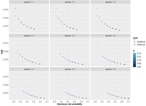
B.2 Upper bound for disclosure risk for multiple passive claimants

While the disclosure risk formula for a passive claimant in a cell with only one passive claimant is useful by itself, it has remarkable implications for the general case of cells with at least one passive claimant, as the following theorem describes. We provide two different proofs of this theorem, one based on the form of the disclosure risk formula and the other on probability theory.

Theorem (Upper bound for the disclosure risk of all passive claimants)
For fixed \(p\in\left(0,\ 1\right),\ q\in\left(0,\ 1\right)\) and \( \epsilon\in\mathbb{R}^{>0}\), an upper bound for the disclosure risk of any passive claimant in a cell with at least one passive claimant is given by,

\(\sup_{R\in\mathbb{R}}{f_{p,\ q,\ \epsilon}\left(R\right)}\)

where

\(f_{p,\ q,\ \epsilon}\left(R\right)=\) (please refer to RHS of Equation b.1.3 from Corollary in B.1.2)

with \( b=-\frac{4}{\epsilon}\ln{\left(1-q\right)}\) and \(c=1-b^2\)

Proof based on the form of the disclosure risk formula

Fix \(p\in\left(0,\ 1\right),\ q\in(0,\ 1) \) and \( \epsilon\in\mathbb{R}^{>0}\). Consider intruder scenario 1 where unit \(k\) (intruder) tries to estimate the value of unit \(j\) (passive claimant) in a cell with only one passive claimant and with units  \(1,2,...,n\) (includes \(j\) and \(k\)) as contributors. Let the true values of the contributors be \(y_1,\ y_2,\ \ldots,\ y_n\).

The results from the previous section says the disclosure risk for unit \(j\) is \(f_{p,\ q,\ \epsilon}\left(R_j\right)\), where \(R_j=\frac{\sum_{i=1,\ i\neq j,\ k}^{n}y_i}{y_j}\). The univariate function \(f_{p,\ q,\ \epsilon}\left(R\right)\) has the graph \(G_{p,\ q,\ \epsilon}=\left\{\left(R,\ f_{p,\ q,\ \epsilon}\left(R\right)\right)\middle| R\in\mathbb{R}\right\}\). The disclosure risk for unit \(j\) corresponds to the point \(\left(R_j,\ f_{p,\ q,\ \epsilon}\left(R_j\right)\right)\) on \(G_{p,\ q,\ \epsilon}\).

Consider intruder scenario 2 which is identical to intruder scenario 1 except unit \(l (\neq j)\) is also a passive claimant whose value is perturbed by log-Laplace multiplicative perturbation. Perturbation of \(y_l\) does not change the function \(f_{p,\ q,\ \epsilon}\) or its graph \(G_{p,\ q,\ \epsilon}\). It merely changes Rj \(R_j\) to a random \(R_j^\prime\in\mathbb{R}\), in which case the disclosure risk of unit \(j\) becomes \(f_{p,\ q,\ \epsilon}\left(R_j^\prime\right)\). This change corresponds to a movement from \(\left(R_j,\ f_{p,\ q,\ \epsilon}\left(R_j\right)\right)\) to \(\left(R_j^\prime,\ f_{p,\ q,\ \epsilon}\left(R_j^\prime\right)\right)\) along graph \(G_{p,\ q,\ \epsilon}\) but does not change \(G_{p,\ q,\ \epsilon}\), which depends only on \(p,q\) and \(\epsilon\) and not on the true or perturbed values of the contributors.

Figure B.2.1 illustrates this for the case where \(p=0.15, q=0.15\) and \(\epsilon=1.3\),

G_pqe (p = 0.15, q = 0.15, e = 1.3)

Figure B.2.1
Graph shows the relationship between the ratio of unprotected contributors to a single protected contributor in an aggregate (x-axis) and the risk of a disclosure under the p% rule (y-axis). The risk increases in the neighbourhood of 0. Two points on the graph show how perturbation of the protected contributor lowers the disclosure risk.

Figure B.2.1: Unit \(j\) has risk \(f_{p,\ q,\ \epsilon}\left(R_j\right)\) if it is the only passive claimant in its cell. Its risk changes to \(f_{p,\ q,\ \epsilon}\left(R_j^\prime\right)\) in the presence of another passive claimant in its cell. This corresponds to movement from the black point to the blue point along the graph \(G_{p,\ q,\ \epsilon}\).

The same conclusion from intruder scenario 2 holds symmetrically for unit \(l\) if unit \(k (\neq l)\) is trying to estimate the value of unit \(l\) instead. That is, unit \(l\) has disclosure risk \(f_{p,\ q,\ \epsilon}\left(R_l^\prime\right)\) instead of \(f_{p,\ q,\ \epsilon}\left(R_l\right)\) in the presence of passive claimant \(j\), but the disclosure risk varies along the same graph \(G_{p,\ q,\ \epsilon}\). This conclusion extends to scenarios with more passive claimants. Since the disclosure risk of any passive claimant only varies along graph \(G_{p,\ q,\ \epsilon}\), every passive claimant in a cell with at least one passive claimant has disclosure risk that is upper bounded by \(\sup_{R\in\mathbb{R}}{f_{p,\ q,\ \epsilon}\left(R\right)}\), which corresponds to the highest point (attained or not) on graph \(G_{p,\ q,\ \epsilon}\).

Proof via probability theory

We previously defined disclosure risk of passive claimant j in a cell with only one passive claimant as,

\(P\left(\left(1-p\right)y_j<{ce}^Xy_j+\sum_{i=1,\ i\neq j,k}^{n}y_i<\left(1+p\right)y_j\middle| p,\ q,\ \epsilon,\ y_1,\ \ldots,\ y_n\right) \tag*{}\)

Note that we now condition on \(p,\ q,\ \epsilon,\ y_1,\ \ldots,\ y_n \) instead of \(p,b,\ \mu,\ y_1,\ \ldots,\ y_n\). This is because \(b\) is a function of \(q\) and \(\epsilon\), and we assume \(\mu=0\) and exclude it for simplicity. Additionally, \(c\)  is a function of \(b\) and therefore a function of \(q\) and \(\epsilon\). Conditioning on \(q\) and \(\epsilon\) instead of \(b\) and \(c\) merely serves as a reminder that disclosure risk is controlled by parameters \(q\) and \(\epsilon\) (as well as \(p\)) from the definition of Pufferfish privacy for q% intervals. We can express the above as,

\(P\left(I\left[\ln{\left(1-p-R\right)}-\ln{\left(c\right)}\right]<X<I\left[\ln{\left(1+p-R\right)-\ln{\left(c\right)}}\right]\middle| p,\ q,\ \epsilon,\ R\right) \tag*{}\)

where \( R=\frac{\sum_{i=1,\ i\neq j,\ k}^{n}y_i}{y_j}\) and \(I(z) = \begin{cases} z &if\ z\in\mathbb{R} \\ -\infty &otherwise \end{cases}\)

Let \(g_{X|R}\left(x\right)\) be the probability density function (pdf) for \(X\) conditioned on \(p, q, \epsilon\) and \(R\). We omit \(p, q\) and \(\epsilon \) from the notation for simplicity, and use \(g\) instead of \(f\) or \(p\) because the two letters already used elsewhere. The disclosure risk for passive claimant \(j\) can be re-expressed as,

\(\int_{I\left[\ln{\left(1-p-R\right)-\ln{\left(c\right)}}\right]}^{I\left[\ln{\left(1+p-R\right)}-\ln{\left(c\right)}\right]}{g_{X|R}\left(x\right)dx} \tag*{}\)

If there are more passive claimants, \(R\) becomes random. \(X\) and \(R\) are independent but this is not important for the proof. Let \( g_R\left(r\right) \) be the pdf for \(R\) and \(g_{X,\ R}\left(x,\ r\right)\) be the joint pdf for \(X\) and \(R\). The disclosure risk for passive claimant \(j\) is then,

\(P\left(I\left[\ln{\left(1-p-R\right)-\ln{\left(c\right)}}\right]<X<I\left[\ln{\left(1+p-R\right)}-\ln{\left(c\right)}\right],\ -\infty<R<\infty\middle| p,\ q,\ \epsilon\right) \\ =\int_{-\infty}^{\infty}\int_{I\left[\ln{\left(1-p-R\right)-\ln{\left(c\right)}}\right]}^{I\left[\ln{\left(1+p-R\right)}-\ln{\left(c\right)}\right]}{g_{X,\ R}\left(x,\ r\right)dxdr} \\ =\int_{-\infty}^{\infty}\int_{I\left[\ln{\left(1-p-R\right)}-\ln{\left(c\right)}\right]}^{I\left[\ln{\left(1+p-R\right)-\ln{\left(c\right)}}\right]}{g_{X|R}\left(x\right)g_R\left(r\right)dxdr} \\ =\int_{-\infty}^{\infty}{g_R\left(r\right)\int_{I\left[\ln{\left(1-p-R\right)}-\ln{\left(c\right)}\right]}^{I\left[\ln{\left(1+p-R\right)-\ln{\left(c\right)}}\right]}{g_{X|R}\left(x\right)dxdr}} \\ let\ M=\sup_{R\in\mathbb{R}}{\int_{I\left[\ln{\left(1-p-R\right)-\ln{\left(c\right)}}\right]}^{I\left[\ln{\left(1+p-R\right)-\ln{\left(c\right)}}\right]}{g_{X|R}\left(x\right)dx}} \\ i.e. \ M=\sup_{R\in\mathbb{R}}{f_{p,\ q,\ \epsilon}\left(R\right)}. \ Continuing \ from\ above, \\ \le\int_{-\infty}^{\infty}{Mg_R\left(r\right)dr} \\ =M\int_{-\infty}^{\infty}{g_R\left(r\right)dr} \\ =M \)

                                                                                                                                                                                         ∎

Remark. Deriving a closed formula for the upper bound described in the theorem above involves examining many cases (5 cases from the piecewise nature of \(f_{p,\ q,\ \epsilon}\) multiplied by multiple cases for the value \(b\)). Further, some equations involving derivatives of \(f_{p,\ q,\ \epsilon}\) seem unsolvable analytically. In practice, it suffices to graph \(f_{p,\ q,\ \epsilon}\left(R\right)\) for some chosen \(p\in\left(0,\ 1\right), q\in\left(0,\ 1\right)\) and \(\epsilon\in\mathbb{R}^{>0}\) (e.g. Figure B.2.1) and graphically approximate the upper bound from the highest point on the graph.

Appendix C - Relative positions of q% intervals proof

 Lemma 3.2.1. The following inequalities, which describe the relative positions of adjacent \(q\)% intervals and adjacent intervals formed by factor \(1-q\), hold for all \(q\in\left(0,1\right)\).

\(1+q\le \frac{1}{1-q} \\ \frac{1}{1-q}\le \frac{\left(1+q\right)^2}{1-q} \\ \frac{\left(1+q\right)^2}{1-q}\le \frac{1}{\left(1-q\right)^3}\)

Proof

We first prove \(1+q\le \frac{1}{1-q}\). The proof is motivated by working backwards from the inequality.

\(-q^2\le0 \\ 1-q^2\le1 \\ \left(1+q\right)\left(1-q\right)\le1 \\ 1+q\le \frac{1}{1-q}\)

We now prove \(\frac{1}{1-q}\le\frac{\left(1+q\right)^2}{1-q}\). The proof is motivated by working backwards from the inequality.

\(0\le q^2+2q \\ 1\le q^2+2q+1 \\ 1\le\left(q+1\right)^2 \\ \frac{1}{1-q}\le\frac{\left(q+1\right)^2}{1-q}\)

We now prove \(\frac{\left(1+q\right)^2}{1-q}\le\frac{1}{\left(1-q\right)^3}\). The proof is motivated by working backwards from the inequality.

\(q^2\left(q^2-2\right)\le0 \\ q^4-2q^2\le0 \\ q^4-2q^2+1\le1 \\ \left(1-q^2\right)^2\le1 \\ \left(1+q\right)^2\left(1-q\right)^2\le1 \\ \left(1+q\right)^2\le\frac{1}{\left(1-q\right)^2} \\ \frac{\left(1+q\right)^2}{1-q}\le\frac{1}{\left(1-q\right)^3} \\\)

Back to top of the page