- For a detailed discussion of price index theory and internationally recommended practices, see Consumer Price Index Manual, Theory and Practice, 2004 (International Labour Office).
- 2 This is the terminology used by Pollak (1971).
- In this example, the price relative shows the change in price between two times. If, instead of two different periods we looked at the price between two different markets in the same period, the price relative would show the difference between the prices in the two markets in the same period.
- The use of the geometric mean of the Laspeyres and Paasche indexes was first proposed by Pigou in 1920, and given the title "ideal" by Fisher (1922).
- For further discussion of forward and backward Laspeyres and Paasche price and quantity indexes, refer to Chapter 2 of Allen (1975).
- Economists measure the change in the quantity of an item in response to a change in price (or income) by elasticities, which are measured as the ratio of the percentage change in the quantity to the percentage change in price (or income). An item is price inelastic if the percentage change in the quantity is less than the percentage change in price. It has unit elasticity if the percentage changes are the same, and is price elastic if the percentage change in the quantity is greater than the percentage change in price. If an item is price inelastic, the change in expenditure will be in the same direction as the change in price (i.e. if price increases, then expenditure also increases). If the item has unit elasticity, then expenditure is unchanged. If the item is price elastic, the change in expenditure will be in the opposite direction to the price change (i.e. if price increases, then expenditure decreases).
- The relationship between the Laspeyres and Paasche indexes holds while there is a normal relationship (negative correlation) between prices and quantities; that is, quantity declines if price increases between the two periods, and vice versa.
- The implicit weights applied by the three formulas are equal base–period quantities (RAP), equal base–period expenditures (quantities inversely proportional to base–period prices) (APR) and equal expenditure shares in both periods (GM).
- The geometric mean of n numbers is the nth root of the product of the numbers. For example, the geometric mean of 4 and 9 is 6 (= ), but the arithmetic mean is 6.5 ( = (4+9)/2 ).
- For a mathematical proof of this see Diewert (1995). The unweighted indexes will all produce the same result if all prices move in the same proportion (have the same relative). In addition, the RAP and APR will produce the same index number if all base–period prices are equal. Diewert also refers to other studies that compare real world results for elementary aggregate formulas.
- For example, Woolford (1994) calculated these indexes for twenty three fresh fruit and vegetable elementary aggregates of the Australian CPI over the period June 1993 to June 1994. He found that the GM produced the lowest increase in sixteen of the twenty three elementary aggregates, and the APR produced the highest increase for nineteen of the elementary aggregates. The RAP formula produced the middle estimate for thirteen of the elementary aggregates. Combining the elementary aggregates to produce the fresh fruit and vegetables index, the index compiled using the APR estimates was 4.7 per cent higher than the index based on GM estimates, and the RAP was 1.7 per cent higher than the index based on GM.
- See Diewert (1995) for further discussion of unit values.
- In a volume index, prices are held constant between the two periods, and the actual quantities from each period are used in the calculation. The change in the index is then measuring the weighted change in the volume of purchases, expenditure etc.
- The characteristics approach to goods is the basis of the so–called household production theory. The development of this theory is generally attributed to Lancaster (1966), Muth (1966) and Becker (1965). Bresnahan and Gordon (1998) also provide a good example using household lighting, tracing the development from whale–oil lamps through to the electric light–bulb, pointing out how the additional inputs required on the part of households (such as trimming wicks etc.) were an important part of the production of light.
- This point, and the use of characteristics in compiling consumer and producer price indexes, are explained in Triplett (1983).
- Pollak (1983) identifies two characteristics approaches, that of Lancaster (1966) and Houthakker (1952). The Lancaster approach assumes that characteristics are additive across items (e.g. protein from meat can be added to protein from bread) whereas the Houthakker approach assumes characteristics are commodity specific.
- There are many examples in literature of the application of the hedonic technique; for example, Ohta and Griliches (1975). For an overview of household production theory and the hedonic technique, see Muellbauer (1974). Pollak (1983) provides an exposition on the treatment of quality in a cost–of–living index.
- For example, the hedonic technique is now used for estimating pure price change for personal computers and television sets in the United States CPI, and personal computers in Australia.
- It is a moot point whether the increased speed and power of computers is reflected in corresponding increases in consumer utility, which raises questions as to whether the hedonic approach adequately captures quality change from a consumer perspective. However, studies have shown remarkable similarities in price indexes based on a hedonics approach and those for computers based on a comprehensive matched models approach.
- Current thinking as presented in Koskimaki and Vartia (2001) for example is that hedonic equations should have log price as the dependent variable and should be estimated for each period. The use of weighted regressions is also supported by researchers such as Diewert. <back
- This is often referred to as the Boskin Report, see Boskin (1996). Boskin estimated that the United States CPI was biased upwards by about 1.1 percentage points a year. There were many submissions and views expressed about bias in the US CPI. For a semi–official perspective on the issue see Moulton (1996).
- As noted earlier, the issue of frequency of re–weighting or chaining is not straightforward. In a situation of price bouncing, chaining can introduce substantial bias into indexes (see for example Szulc (1983)). In general, chaining more frequently than annually, even if feasible in practice, is not recommended because it could introduce bias.
This is not the latest release View the latest release
Consumer Price Index: Concepts, Sources and Methods
This release provides updated information relating to the data sources and methods used to compile the CPI
Reference period
2018
Released
27/02/2019
Aim of this publication
1.1 The Australian Consumer Price Index (CPI) is an important economic indicator. It measures price changes experienced by households. It is compiled according to international standards, and is based on robust data collection and compilation methodologies. This publication provides a comprehensive description of price index theory and methodology, focusing on the Australian CPI and the concepts, sources and methods behind its compilation. It also provides some insight into the kinds of conceptual and practical difficulties that the Australian Bureau of Statistics (ABS) encounters in compiling the CPI, and how it deals with these challenges.
1.2 The ABS currently publishes a set of Frequently Asked Questions (FAQs) and a brief description of the CPI in A Guide to the Consumer Price Index: 17th Series, 2017 (cat. no. 6440.0). The Guide is for those interested in a straightforward and brief account of the main features of the CPI. This Concepts, Sources and Methods publication, on the other hand, is for those users who require a deeper understanding of the CPI, and of the methods and techniques used to deal with the complex situations that arise in constructing price indexes across the spectrum of household consumer expenditure.
Other sources of information about the Consumer Price Index
1.3 The CPI is compiled quarterly by the ABS for quarters ending on 31 March, 30 June, 30 September, and 31 December each year. The CPI is released each quarter on the last Wednesday of the month following the end of the reference quarter, depending on public holidays, in the publication Consumer Price Index, Australia (cat. no. 6401.0).
1.4 From December quarter 2017, the CPI is re-weighted annually. The Household Expenditure Survey (HES) is used to update the weights in the years that it is available. For the inter-HES years, Household Final Consumption Expenditure (HFCE) data from the National Accounts is used as the principal data source for re-weighting the CPI. Prior to this, the CPI was reviewed and re-weighted every six years. The ABS described the change to annual re-weighting in the following information papers:
- Information Paper: Increasing the Frequency of CPI Expenditure Class Weight Updates, July 2016 (cat. no. 6401.0.60.002); and
- Information Paper: An Implementation Plan to Annually Re-weight the Australian CPI, 2017 (cat. no. 6401.0.60.005).
1.5 The 17th series used data from the Household Expenditure Survey, Australia: Summary of Results, 2015-16 (cat. no. 6530.0) to represent household expenditure patterns. It was introduced in the December quarter 2017 following a minor review. As well as updating the weights in the CPI basket, the review included a simple examination of structures and methodologies. As part of the 17th series review, the ABS published an Information Paper:
- Information Paper: Introduction of the 17th Series Australian Consumer Price Index, 2017 (cat. no. 6470.0.55.001).
1.6 The 16th Series CPI introduced in the September quarter 2011 was a major review. The item weights were revised in line with expenditure patterns identified in the 2009-10 Household Expenditure Survey (HES). As well as updating the weights in the CPI basket, the review looked at the uses, concepts and purpose of the CPI and confirmed the principal purpose of the CPI is to measure inflation faced by households to support macroeconomic policy decision making. As part of the 16th series review, the ABS published a number of Information Papers:
- Issues to be considered during the 16th Series Australian Consumer Price Index Review, Dec 2009 (cat. no. 6468.0);
- Outcome of the 16th Series Australian Consumer Price Index Review, Dec 2010 (cat. no. 6469.0); and
- Information Paper: Introduction of the 16th Series Australian Consumer Price Index, 2011 (cat. no. 6470.0).
1.7 These papers describe the review process, the issues considered, the review outcomes, the re-weighting process and outline the changes from the previous series.
1.8 The 15th Series CPI introduced in the September quarter 2005 was a minor review. The item weights were revised in line with expenditure patterns identified in the 2003-04 Household Expenditure Survey (HES) and a new sub-group called Financial services was introduced into the CPI. The ABS published an Information Paper describing the changes:
- Information Paper: Introduction of the 15th Series Australian Consumer Price Index, 2005 (Reissue) (cat. no. 6462.0).
1.9 The 14th Series CPI was introduced in the September quarter 2000, after a minor review completed early in 2000. The changes introduced in the 14th series were considered necessary to address issues arising from the introduction of The New Tax System (TNTS) on 1 July 2000. As part of the review process the ABS published two Information Papers describing the changes:
- Information Paper: Price Indexes and The New Tax System, 2000 (cat. no. 6425.0); and
- Information Paper: Introduction of the 14th Series Australian Consumer Price Index, 2000 (cat. no. 6456.0).
1.10 The 13th Series CPI, which followed a major review of the index, was introduced in the September quarter 1998. Several important changes were made to the index at that time. Prior to the September quarter 1998, the CPI was compiled primarily to be used for income adjustment through wage indexation. This had implications for the coverage and design of the index. It was limited to the expenditures made by households whose principal source of income was wages. It measured out-of-pocket living expenses, including mortgage interest payments.
1.11 Since the September quarter 1998, the principal purpose of the CPI has been to measure inflation faced by households to support the operation of macroeconomic policy decision making. The CPI covers the expenditures of all households (not just those whose principal source of income is wages, as was the case before 1998) and measures the changes in the prices of a basket of goods and services acquired each period. The cost of housing is measured as the price of a new home (excluding land). Mortgage interest payments are excluded.
1.12 As part of the 13th Series review, the ABS published three Information Papers:
- Information Paper: Issues to be Considered During the 13th Series Australian Consumer Price Index Review, Apr 1997 (cat. no. 6451.0);
- Information Paper: Outcome of the 13th Series Australian Consumer Price Index Review, 1997 (cat. no. 6453.0); and
- Information Paper: Introduction of the 13th Series Australian Consumer Price Index, 1998 (cat. no. 6454.0).
1.13 In recognition of the interest in the extent to which the impact of price change varies across different groups in the community, in addition to the CPI, the ABS compiles the Selected Living Cost Indexes, Australia (cat. no. 6467.0).
Contact details
1.14 The ABS intends to update this manual periodically. Therefore, the ABS would welcome comments from the users of statistics covered in this publication. You may direct your comments or questions to:
Consumer Price Index Section
Australian Bureau of Statistics
Locked Bag 10
Belconnen, ACT, 2616
Telephone: 02 6252 6654
Email: prices.statistics@abs.gov.au
Purposes and uses of consumer price indexes
Introduction
2.1 A consumer price index measures the change in the prices paid by households for goods and services consumed. All expenditure by businesses, and expenditure by households for investment purposes, are out of scope of a consumer price index. In this regard, expenditure on housing presents particular difficulties as it can be considered as part investment and part purchase of shelter-related services.
2.2 There is currently no single, universally accepted definition of a consumer price index. The often quoted description of a CPI is the following statement from the Resolution concerning consumer price indexes released in 2003 by the Seventeenth International Conference of Labour Statisticians convened by the International Labour Organization (ILO) (the Resolution is reproduced in Appendix 4):
"The CPI is a current social and economic indicator that is constructed to measure changes over time in the general level of prices of consumer goods and services that households acquire, use or pay for consumption. The index aims to measure the change in consumer prices over time. This may be done by measuring the cost of purchasing a fixed basket of consumer goods and services of constant quality and similar characteristics, with the products in the basket being selected to be representative of households’ expenditure during a year or other specified period."
Principal purposes of a Consumer Price Index
2.3 A consumer price index may serve several purposes. However, three principal purposes are generally recognised, namely to measure:
- changes in the purchasing power of money incomes;
- changes in living standards; and
- price inflation experienced by households.
Purchasing power of money incomes
2.4 A CPI designed to measure the purchasing power of money incomes is concerned with answering questions such as how much income is required today to purchase the same basket of goods and services that was purchased in the base period. The appropriate domain of the basket in this case is all those outlays on consumer goods and services actually made by households in the base period.
2.5 For this purpose the correct measure of income to use is net income (i.e. after income tax), not gross income. Application of the index to gross income is only valid if income tax is proportional to income, and the treatment of property income is identical to that of wage and salary income. A progressive income tax regime, such as that applying in Australia, emphasises the need to use net income. In addition, as the significance of different sources of income and expenditure varies considerably between household types, changes in purchasing power are best assessed by type of household rather than in total.
Assessing changes in living standards
2.6 In assessing changes in living standards, the CPI is used in conjunction with data on expenditures by households to measure changes in their volume of consumption of all goods and services.
2.7 For this purpose, the first thing to do is to define standard of living. A narrow definition of standard of living is the volume of goods and services consumed by households in the base period. For many consumer items, the acquisition of, the payment for, and the consumption of, an item all occur at about the same time. However, for some items the volume of the item consumed in a period may have little relationship to the payments made in the period. A good example of this is a consumer durable such as a private motor vehicle where the vehicle may have been purchased several years earlier. For other items, the price is substantially below the economic cost of providing the good or service, so that the expenditure is not a true reflection of the quantity of the item consumed. Typical examples of this are services provided by the public sector such as education and medical care. Estimates must be made of the economic value of these items actually consumed in the base period.
2.8 Estimates of the market value of the consumption of consumer durables can be made by reference to the market prices of similar items (thus private rents can be used as an indicator of the value of owner-occupied housing, and leasing charges for households' fleet of motor vehicles). For insurance services, estimates of the service component (essentially operating costs plus profit) are derived from the published accounts of insurance companies. For publicly supplied goods and services, the ABS compares their prices with those of private suppliers of similar services or makes estimates based on the cost of providing the service (e.g. teachers’ salaries plus building and running costs for educational services).
2.9 Of course, a broader definition of living standards is possible. It might include environmental conditions such as the quality of air and water, or the area of national parks. Although these are important in their own right, the measurement of these factors, the value placed on them by households, and the means of including them in an index of living standards, are as yet insoluble problems (see Pollak (1998)). So for practical reasons, the narrow definition is used.
2.10 Against this background, the domain for an index designed to assess changes in living standards would include:
- residential rent payments;
- imputed rent of owner-occupied dwellings;
- consumer durables;
- the value of insurance and banking service charges;
- other private-sector goods and services; and
- government-provided goods and services valued at cost or at their estimated market prices.
2.11 This measure accords with the concept of Household Final Consumption Expenditure (HFCE) in the Australian National Accounts.
Measuring household inflation
2.12 Another possible purpose of the CPI is to measure household inflation. This measure is primarily for use in macroeconomic management, and also has some possible uses in contracts where an index of prices for household consumption items is appropriate. Of course, as the CPI measures only households' price experience, it is not a measure of economy-wide inflation.
2.13 As there is no generally agreed definition of inflation, the issue of how it should be measured is complicated. Nevertheless, it seems clear that an index of household inflation should attempt to measure the contemporary rate of change in prices of consumer goods and services.
2.14 An important aspect of a measure of inflation is that it should only include market-determined prices. Thus, an inflation measure would not include imputed rent of owner-occupied dwellings (which, however, would be included in a cost-of-use approach as discussed below). A measure of house prices would be more appropriate, if housing is not considered an investment. Financial assets would not be considered a good or service, thus prices of shares and the like would be out of scope. However, such a measure would need to capture changes in the service charges of intermediaries involved in financial and asset-transaction services, such as banks, insurance companies, and real estate agents
2.15 It could be argued that an inflation measure should also exclude goods and services provided to households at subsidised prices. The reason is that the inflation rate has implications for government policy, and as such it should be determined by market forces unhindered by the actions of governments themselves. The argument goes that subsidies are distortions of pure market forces, and subsidised prices do not reflect the true market price (or economic value) of the goods and services. However, the treatment of taxes, and subsidies which are regarded as negative taxes, should be symmetrical. Excluding subsidised goods would lead to some significant goods and services (e.g. education) being omitted that would otherwise be considered essential for complete coverage in a CPI. Consequently, the most common practice is to include subsidised goods and services.
2.16 The domain for a measure of household inflation would thus include:
- residential rent payments;
- net purchase of owner-occupied dwellings;
- net purchase of consumer durables;
- the value of intermediary services for transactions in real and financial assets (e.g. banking and stockbroking services); and
- other consumer goods and services provided at market prices.
2.17 As it presently stands, the Australian CPI is specifically designed to provide a general measure of price inflation for households residing in the capital cities.
Conceptual approaches to constructing a Consumer Price Index
2.18 Once the purpose of a CPI is decided, a method of construction can be worked out to satisfy that purpose. Consistent with the three purposes outlined above, there are three possible conceptual approaches for constructing a CPI. These approaches are consistent with the ILO Resolution which says that "...a reference population acquires, uses or pays for consumer goods and services".
These are the three methods.
(i) The Acquisitions method: in the base period, all goods and services acquired (i.e. actually received) by the reference population are included in the CPI regardless of the period in which payment or use occurs.
(ii) The Cost-of-Use method: in the base period, all goods and services used (i.e. consumed) by the reference population are included in the CPI regardless of when they are paid for or acquired. In particular, the cost of using the good or service is measured by its true economic cost.
(iii) The Outlays method: in the base period, all goods or services for which payments were made are included in the CPI without regard to the source of the funds.
2.19 The acquisitions and outlays approaches are similar. The acquisitions approach leads to a CPI basket that can be viewed as a subset of the basket resulting from an outlays approach. Both conceptual approaches include goods and services acquired during the base period, but the outlays approach also effectively includes any inescapable costs associated with the acquisition of a good or service, such as interest charges. The cost-of-use approach can result in a basket that differs from both the acquisitions and outlays approaches.
2.20 The choice of conceptual approach for construction of the index depends on the purpose. The approach that is most appropriate for each of the three possible CPI purposes is outlined below.
(i) Purchasing power of money incomes. In order to determine changes in the purchasing power of money, an outlays approach is most appropriate. The outlays approach provides a proxy for household income through measurement of consumer outlays.
(ii) Assessing changes in living standards. The cost-of-use approach provides the best indication of changes in living standards as it relates to goods and services actually consumed in the base period.
(iii) Measuring household inflation. The acquisitions method is the most appropriate for this purpose. A measure of household inflation should relate to the contemporary rate of change in the prices of goods and services. The acquisitions approach captures this by measuring changes in the prices of goods and services actually acquired in the base period.
Comparison of the conceptual approaches
2.21 In practice, for most goods and services purchased by the reference population, outlay, acquisition, and use all occur within a short period, and the price paid by the reference population is a true economic value, effectively making the distinction between the approaches academic. However, in some cases there can be significant lags between outlay, acquisition, and use; or the price paid may differ significantly from what is considered the true value.
2.22 There are three areas of household expenditure in which these conceptual approaches provide significantly different results. These are:
(i) the purchase of housing;
(ii) the purchase of durable goods; and
(iii) financial services, including the use of credit.
2.23 To illustrate the differences among the three approaches, the way in which these three special cases are treated under each approach is outlined below.
Expenditure on housing
2.24 Under the acquisitions approach, the required measure is the change in prices for both the net purchase of housing, and the increase in the volume of housing because of renovations and extensions, plus other costs incurred in ensuring the continued supply of services provided by owner-occupied dwellings (e.g. maintenance costs and council rates). Changes in rents are measured for that part of the reference population that resides in rented dwellings. Costs such as maintenance of rental dwellings are paid by investors who are out of scope of a CPI.
2.25 Under the outlays approach, the required measure includes changes in the amount of interest paid on mortgages, and the costs incurred in ensuring the continued supply of services provided by the dwellings (e.g. maintenance costs and council rates). Also included are changes in rents which are measured for that part of the reference population that resides in rented dwellings.
2.26 Under the cost-of-use approach, the required measure is the change in the economic value of the services provided by dwellings. The price of these services is usually measured as the rental value of the dwellings. For owner-occupied dwellings, the rental values are imputed. Costs such as maintenance costs are not included as they are part of the cost of maintaining an investment, and so are outside the scope of a CPI.
Durable goods
2.27 For durable goods, the three approaches result in the following treatments
(i) Acquisitions - the basket includes those durable goods acquired in the base period, and their price measure is the transaction (purchase) price.
(ii) Outlays - the basket includes those durable goods paid for in the base period, and their price measure is the transaction price.
(iii) Cost-of-use - the basket includes the services of durable goods consumed in the base period, regardless of the period in which they were purchased, and the price measure is the market value of the services provided by those goods (measured in business accounts as depreciation plus the return on investment).
Financial services and the use of credit
2.28 Under the acquisitions approach, interest paid is not a charge that is within scope of the CPI basket of goods and services. The service for which prices are required is that of providing banking services (including the provision of loans).
2.29 Under the outlays approach, the product being priced is the cost of servicing loans taken out to purchase products that are part of the CPI basket. Thus the change in the level of interest paid on this debt is the required price measure.
2.30 The cost-of-use approach requires that the cost of the financial services used is measured in a similar manner to the acquisitions approach.
Concluding remarks
2.31 The alternate approaches to the construction of the CPI reflect conceptual differences; and their use is determined by the purpose of the CPI.
The Australian Consumer Price Index
1997 Review and the adoption of an acquisitions basis for the CPI
2.32 In 1997 a major review of the CPI was conducted, involving consultation with a wide range of organisations and individuals representing government, social, business and community interests. This review concluded that the ABS should change from an outlays index for wage and salary earner households and adopt an acquisitions approach as a general measure of household inflation for all private households. Since the introduction of the 13th series CPI in the September quarter 1998, the CPI has been compiled on an acquisitions basis. Another major review of the CPI was conducted in 2010 which concluded that, with the introduction of the 16th series CPI, the acquisitions approach continue to be used in the compilation of the CPI. For more detail on the 1997 and 2010 Reviews, see:
- Information Paper: Issues to be Considered During the 13th Series Australian Consumer Price Index Review, Apr 1997 (cat. no. 6451.0);
- Information Paper: Outcome of The 13th Series Australian Consumer Price Index Review, 1997 (cat. no. 6453.0);
- Information Paper: Introduction of the 13th Series Australian Consumer Price Index, 1998 (cat. no. 6454.0);
- Information Paper: Issues to be considered during the 16th Series Australian Consumer Price Index Review, Dec 2009 (cat. no. 6468.0);
- Information Paper: Outcome of the 16th Series Australian Consumer Price Index Review, Australia, December 2010 (cat. no. 6469.0); and
- Information Paper: Introduction of the 16th Series Australian Consumer Price Index, 2011 (cat. no. 6470.0).
Uses of the CPI
2.33 A major use of the CPI is to assist government economists in conducting general economic policy, especially monetary policy. Since 1993, Australian monetary policy has been conducted with the aim of meeting a medium-term inflationary target. Since the introduction of the 13th series CPI in the September quarter 1998, that target has been the inflation rate as measured by the CPI. Additional analytical series including the international trade exposure and underlying trend estimates are also used to assist in understanding inflationary trends.
2.34 The CPI, or one of its components, is also widely used in indexation arrangements in both the private and public sectors. These include indexing pension and superannuation payments, taxes and charges, some governmental bonds, and business contracts.
2.35 In Australia, the use of the CPI in wage determination has diminished with the trend towards decentralised, enterprise-based wage and salary setting arrangements with outcomes focused on the commercial circumstances of each business.
Historical background
Introduction
3.1 Before the introduction of the Consumer Price Index (CPI) in 1960, there were five series of retail-price indexes compiled by the then Commonwealth Bureau of Census and Statistics. Those indexes were as follows:
(i) The A Series Index, covering only food, groceries and housing rents (for all houses), which was first compiled in 1912 with index numbers going back to 1901, was discontinued in 1938. Its main use was for adjusting wages between 1913 and 1933.
(ii) The B Series Index, covering only food, groceries and housing rents (for four and five-roomed houses), which was first compiled in 1925, was discontinued in 1953. It was introduced to replace the A Series Index for general statistical purposes, but was never used for adjusting wages.
(iii) The C Series Index, covering food and groceries, housing rents (for four and five-roomed houses), clothing, household drapery, household utensils, fuel, lighting, urban-transport fares, smoking and some miscellaneous items, which was introduced in 1921, was discontinued in 1961. The food and rent component of the C Series Index was the same as that for the B Series Index. The C Series Index was used to adjust wages from 1934 until it was discontinued.
(iv) The D Series Index, which was derived by combining the A Series and C Series Indexes, and was compiled especially for wage adjustment purposes for a short period in 1933-34.
(v) The Interim Retail Price Index, covering food and groceries, housing rents (for four and five-roomed houses), clothing, household drapery, household utensils, fuel, lighting, urban-transport fares, smoking, and some services and miscellaneous items which was first compiled in 1954 and was discontinued in 1960. As the name implies, the Interim Index was intended to serve as a transitional index, but to some extent it replaced the C Series Index for general statistical purposes for a few years before 1960. It was never used for wage adjustment purposes.
C Series Index
3.2 By far the most important of these old price indexes was the C Series Index which was the principal retail price index in Australia for almost forty years. It was first compiled in 1921 with index numbers compiled back to 1914. C Series Index numbers were compiled for:
(i) the capital city in each of the six states;
(ii) four of the larger towns in each of the six states;
(iii) weighted average of five towns (including the capital city) in each of the six states;
(iv) weighted average of the six state capital cities;
(v) weighted average of thirty towns (including the capital cities); and
(vi) three additional towns - Whyalla, Port Augusta, and Canberra.
3.3 The C Series Index was reviewed in 1936 and a slightly revised selection of goods and services was introduced, which then remained unchanged until the C Series Index was discontinued.
3.4 The main reason for the long interval without any review or change in composition of the C Series Index after 1936 was the recurrent changes in consumption patterns which occurred during and after World War II. It was considered impossible at the time to devise a revised weighting pattern which would be any more representative of post-war consumption than the existing weighting pattern of the C Series Index. The Commonwealth Statistician of the time, in successive editions of the Labour Report during the 1950s and 1960s, explained the absence of any re-weighting of the C Series Index in the following words.
"From the outbreak of war in 1939 to late in 1948, periodic policy changes in various wartime controls (including rationing) caused recurrent changes in consumption and in the pattern of expenditure. This rendered changes desirable but made it impracticable either to produce a new index, or to revise the old one, on any basis that would render the index more representative than it already was of the changing pattern of household expenditure in those years. When commodity rationing had virtually ceased in the latter part of 1948 action was taken by the Statistician to collect price data of about 100 additional items and to gather information as to current consumption and expenditure patterns. This was done to facilitate review of the component items and weighting system of the C Series Retail Price Index in the light of the new pattern of wage earner expenditure and consumption that appeared to be then emerging. But there supervened, in the next few years, conditions which caused wide price dispersion, coupled with a very rapid rise in prices and a new sequence of changes in consumption and in the pattern of wage earner expenditure. Under these conditions it was not possible to devise any new weighting pattern likely to be more continuously representative of conditions then current, than was the existing C Series Index on the 1936 revision."
3.5 In 1953, the decision was made to continue compiling the C Series Index on its pre-war basis, but also to compile an interim retail price index based as nearly as possible on the post-war pattern of consumer usage and expenditure. Nevertheless, the C Series Index continued to be regarded by the majority of users as the principal official index, and was the one used in most indexation and escalation arrangements throughout the 1950s.
Interim Retail Price Index
3.6 The Interim Retail Price Index was based on post-war consumption weights. Compared with the C Series Index, the Interim Index covered an expanded range of items, including additional foods (such as packaged breakfast foods, soft drinks, ice cream, and confectionery) and services (such as dry-cleaning and shoe repairs). Throughout the period of its compilation, no attempt was made to revise its weights to take account of major changes in expenditure patterns and lifestyles that were occurring during the 1950s. During that decade, house renting was substantially replaced by home ownership, the use of motor cars partially replaced the use of public transport, and a variety of electrical appliances, and subsequently television, became widely used by households. During the same period, widely disparate movements occurred in the prices of different items routinely purchased by households. It was considered that the combined effect of these factors made it impracticable to introduce a comprehensive new retail price index during the period to 1960.
Consumer Price Index
3.7 In 1960, a new approach was tried. Instead of the former emphasis on long-term fixed-weighted indexes, the aim was to compile a series of shorter term indexes that would be chain linked to form long-term series. The Consumer Price Index, commonly referred to as the CPI, was the first price index of this kind constructed in Australia.
3.8 The CPI was first compiled in 1960 with index numbers compiled back to mid-1948. Like the old indexes, the CPI was designed to measure quarterly changes in the retail prices of goods and services purchased by metropolitan wage-earning households.
3.9 At its inception in 1960, the CPI consisted of three original series linked together with changes in weights in 1952 and 1956. Weights were changed in 1960 and subsequently in 1963, 1968, 1973, 1974, 1976, 1982, 1987, 1992, 1998, 2000, 2005, 2011 and 2017. From 2017, the CPI is re-weighted annually each December quarter. The Household Expenditure Survey (HES) is used to update the weights in the years that it is available. For the inter-HES years, Household Final Consumption Expenditure (HFCE) data from the National Accounts is used as the principal data source for re-weighting the CPI.
Long-term linked series
3.10 To provide an approximate long-term aggregate measure of consumer price change for the period since the first Australian retail price index was compiled, the ABS has constructed a single series of index numbers by linking together selected retail and consumer price index series from amongst those described above (see Table 3.1). The index numbers are expressed with an index reference base of 1945 equals 100.0 which was the end of a period of price stability during World War II. The successive series linked together to produce this long-term series of index numbers are:
- from 1901 to 1914, the A Series Retail Price Index;
- from 1914 to 1946-47, the C Series Retail Price Index;
- from 1946-47 to 1948-49, a combination of the C Series Index, excluding the housing group of the CPI; and
- from 1948-49 onwards, the CPI.
3.11 This long-term series of index numbers is updated each year. A graph of the series taken from Table 3.1 is presented in Figure 3.1.
| Year | Index | Year | Index | Year | Index | Year | Index |
|---|---|---|---|---|---|---|---|
| 1901 | 47 | 1931 | 78 | 1961 | 252 | 1991 | 1,898 |
| 1902 | 50 | 1932 | 74 | 1962 | 251 | 1992 | 1,917 |
| 1903 | 49 | 1933 | 71 | 1963 | 252 | 1993 | 1,952 |
| 1904 | 46 | 1934 | 73 | 1964 | 258 | 1994 | 1,989 |
| 1905 | 48 | 1935 | 74 | 1965 | 268 | 1995 | 2,082 |
| 1906 | 48 | 1936 | 75 | 1966 | 276 | 1996 | 2,136 |
| 1907 | 48 | 1937 | 78 | 1967 | 286 | 1997 | 2,141 |
| 1908 | 51 | 1938 | 80 | 1968 | 293 | 1998 | 2,159 |
| 1909 | 51 | 1939 | 82 | 1969 | 302 | 1999 | 2,191 |
| 1910 | 52 | 1940 | 85 | 1970 | 313 | 2000 | 2,289 |
| 1911 | 53 | 1941 | 89 | 1971 | 332 | 2001 | 2,389 |
| 1912 | 59 | 1942 | 97 | 1972 | 352 | 2002 | 2,462 |
| 1913 | 59 | 1943 | 101 | 1973 | 385 | 2003 | 2,530 |
| 1914 | 61 | 1944 | 100 | 1974 | 443 | 2004 | 2,588 |
| 1915 | 70 | 1945 | 100 | 1975 | 510 | 2005 | 2,658 |
| 1916 | 71 | 1946 | 102 | 1976 | 579 | 2006 | 2,753 |
| 1917 | 75 | 1947 | 106 | 1977 | 650 | 2007 | 2,817 |
| 1918 | 80 | 1948 | 117 | 1978 | 702 | 2008 | 2,940 |
| 1919 | 91 | 1949 | 128 | 1979 | 766 | 2009 | 2,994 |
| 1920 | 103 | 1950 | 140 | 1980 | 844 | 2010 | 3,079 |
| 1921 | 90 | 1951 | 167 | 1981 | 926 | 2011 | 3,181 |
| 1922 | 87 | 1952 | 196 | 1982 | 1,028 | 2012 | 3,237 |
| 1923 | 89 | 1953 | 205 | 1983 | 1,132 | 2013 | 3,316 |
| 1924 | 88 | 1954 | 206 | 1984 | 1,177 | 2014 | 3,399 |
| 1925 | 88 | 1955 | 211 | 1985 | 1,257 | 2015 | 3,450 |
| 1926 | 90 | 1956 | 224 | 1986 | 1,370 | 2016 | 3,494 |
| 1927 | 89 | 1957 | 229 | 1987 | 1,487 | 2017 | 3,562 |
| 1928 | 89 | 1958 | 233 | 1988 | 1,594 | 2018 | 3,630 |
| 1929 | 91 | 1959 | 237 | 1989 | 1,714 | ||
| 1930 | 87 | 1960 | 245 | 1990 | 1,839 |
- Base: Calendar Year 1945 = 100.0.
- The index numbers relate to the weighted average of six state capital cities from 1901 to 1980 and to the weighted average of eight capital cities from 1981. Index numbers are for calendar years.
- Any discrepancies with movements published in ABS cat. no. 6401.0 are due to different index reference periods and rounding.
Price index theory
Overview
4.1 Price indexes in one form or another have been constructed for several centuries, and are commonly used in everyday life. However, the complexities of price indexes are not always fully appreciated or understood. Price index theory provides an overview of the theory and practices that underpin the construction of price indexes.¹
4.2 Price index theory commences by describing the concept of a price index as a single-number representation of information about many prices before discussing the relationship between indexes of prices, quantities and expenditures.
4.3 Two levels of construction of price indexes are described. At the lowest level is the construction of an index for a narrowly defined commodity from price observations. The other is the aggregation of these basic or elementary aggregate indexes across a range of commodities. Various mathematical formulas for constructing these indexes are discussed including problems for prices statisticians in selecting the most appropriate methodology. The advantages and disadvantages of the various formulas are discussed, along with criteria to guide decisions on the most appropriate formula.
4.4 Price index theory concludes with a discussion of issues that arise in price index construction, including changes in observation numbers, quality adjustments, the inclusion of new products and index number bias.
4.5 Price index theory focuses on traditional price index methods, however in the past ten years there have been significant developments in new price index construction methods involving transactions (scanner) data. These methods are discussed in more detail in Use of transactions data in the Australian CPI of this manual.
The concept of a price index
Comparing prices
4.6 There are many situations where there is a need to compare two (or more) sets of price observations. For example, a household might want to compare prices today with some earlier period; a manufacturer would be interested in comparing prices between markets to determine where to sell its output, or to compare price movements between two time periods with movements in its production costs; and economists and market analysts need to be able to compare prices between countries and over time to assess and forecast a country’s economic performance.
4.7 In some situations, the price comparisons might only involve a single commodity. Here it is simply a matter of directly comparing the two price observations. For example, a household might want to assess how the price of shampoo today compares with the price at some previous time for the same item.
4.8 In other circumstances, the required comparison is of prices across a range of commodities. For example, a comparison of clothing prices might be required. There is a wide range of clothing types and thus prices to be considered (e.g. toddlers’ jump suits, women’s fashion skirts, boys’ shorts, men’s suits). Although comparisons can readily be made for individual or identical clothing items, this is unlikely to enable a satisfactory result for all clothing in aggregate. A method is required for combining the prices across this diverse range of items allowing for the fact that they have many different units or quantities of measurement. This is where price indexes play an extremely useful role.
The basic concept
4.9 A price index allows the comparison of two sets of prices either over time (temporal indexes) or regions (spatial indexes) for a common item or group of items. In order to compare the sets of prices, it is necessary to designate one set the reference set and the other the comparison set.² The reference price set is used as the base (or first) period for constructing the index, and by convention in Australia is always given an index value of 100. For example, suppose for a single item the average of prices in the first set was $15 and for the second set was $30. Then, designating the first set as the reference set gives an index of 200.0 (30/15x100) for the comparison second set. Designating the second set as the reference set gives an index of 50.0 (15/30×100) for the comparison first set.
4.10 The most common price index is a comparison between sets of prices at two times (temporal indexes). The times can be adjacent (this month and previous month) or many periods apart (this year and ten years earlier). Typically the method is to nominate one set of prices as the reference prices and to revalue the quantities (or basket) of items purchased in the base period by prices in the second (or comparison) period. The ratio of the revalued comparison period basket to the value of the reference period basket provides a measure of the price change between the two periods. This simple revaluation, however, does not take account of any changes or substitutions that may be made in quantities consumed in response to changes in relative prices between the two periods. Nor does it allow for any change in tastes between the two periods. These changes to the preferences of consumers are significant in the choice of index methodology.
4.11 Handling quantity changes that occur in response to changes in relative prices is fundamental to price index construction. Changes in the relative importance of items in the basket of goods and services can have a significant effect on index movements.
4.12 Another objective of price indexes is to determine levels of household expenditure that are equivalent between two cities, say Darwin and Hobart. To do this, a spatial price index is required which allows the price levels in the two cities to be compared. This can be done by specifying a basket (i.e. quantities) of goods and services, and pricing this basket in both cities. The ratio of the total price of the basket in each city gives a measure of price relatives.
4.13 The composition of the basket would depend on the comparison required. For example, suppose the household was considering relocating from Darwin to Hobart and desired to be no worse off in terms of the overall basket of goods and services it could purchase. The reference basket should then comprise the quantities of each item currently purchased by the household in Darwin. Alternatively, if the household were in Hobart and considered relocating to Darwin, then it would specify the reference basket as the quantities of goods and services being purchased in Hobart.
4.14 The composition of the basket reflects the consumption preferences of the subject, in this case the household. It will reflect the household’s preferences under the prices and income prevailing in its current situation. Ideally, what would be required is some indication of how the household’s tastes or preferences might change between locations. Clearly the household could choose a different mix of items in Hobart than in Darwin, reflecting differences in relative prices between the cities, climate and other factors. The objective, though, is the same: to measure the relative expenditures in the two cities for which the household is equally satisfied (or indifferent).
Refining the concept
4.15 The remainder of Price index theory focuses on the comparison of prices over time (temporal indexes). Expenditure on an individual item is the product of price and quantity, that is:
\(e_t = p_tq_t \space \space \space \space \space \space (4.1)\)
where \(e\) is expenditure, \(p\) is price, \(q\) is quantity and the subscript \(t\) refers to the time periods at which the observations are made.
4.16 Consider the expenditures on the same commodity in two different times periods. Changes in these expenditures can reflect changes in the price, changes in the quantity, or a combination of both price and quantity changes. For example, suppose the price of Granny Smith apples at a particular market is $2.00 per kg in period one, and it rises to $2.50 per kg in period two. The change in the price of apples between these two periods is obtained from the ratio of the price in the second period to the price in the first period; that is, $2.50/$2.00 = 1.25 or an increase of 25% in the price. If a consumer bought exactly the same quantity of apples in the two periods, the expenditure on Granny Smith apples would rise by 25%. However, if the amount purchased in the first period was 10 kg, and the amount purchased in the second period was 12 kg, the quantity would also have risen by a factor of 12/10 = 1.20 or 20%. In these circumstances, the total expenditure on apples increases from $20 in the first period (10 kg at $2.00 per kg), to $30 in the second period (12 at $2.50 per kg), an increase in expenditure of $10 or 50%. The ratio of the current expenditure to the previous expenditure is the product of the change in price and the change in quantity (1.25 x 1.20 = 1.50).
4.17 The ratio between the price in the current period and the price in the reference period is called a price relative. A price relative shows the change in price for one item only (e.g. the pricing of Granny Smith apples at one particular fruit market).
In terms of the formula in equation 4.1:
\(e_1\) (expenditure in period 1) = \(p_1\) ($2.00) x \(q_1\) (10kg) = $20, and
\(e_2\) (expenditure in period 2) = \(p_2\) ($2.50) x \(q_2\) (12kg) = $30
where: \(p_1\) is the price per kg in period 1; \(q_1\) is the quantity in period 1;
\(p_2\) is the price per kg in period 2 and \(q_2\) is the quantity in period 2.
The ratio between the prices in the two periods, \(p_2\) and \(p_1\) ($2.50/$2.00 = 1.25) is the price relative.³
4.18 It is only necessary to have observations on two of the three components of equation 4.1 to analyse contributions to change in the expenditure. Using the apple example, suppose observations were only available on expenditure and price. The expenditure could be divided by the price to estimate the quantity (or the movements in expenditure and price could be used). Alternatively, if only expenditure and quantity data were available, expenditure could be divided by quantity to derive what's known as the 'unit (price) value'.
4.19 Now consider the case of price and quantity (and expenditure) observations on many commodities. The quantity measurements can have many dimensions, such as kilograms, tonnes, or even units (e.g. number of motor cars), and the quantities and prices of items are likely to show different movements between periods. Answers are required to questions such as these: what is the change over time in the quantity of commodities, and what is the contribution of price changes to changes in the expenditure on the bundle of commodities over time? Answering these questions is the task of index numbers: to summarise the information on sets of prices and quantities into single measures to assist in understanding and analysing changes.
4.20 In essence, an index number is an average of either prices or quantities compared with the corresponding average in a base period. The problem is how to calculate the average.
4.21 More formally, the price index problem is how to derive an index of price \((I^P)\) and an index of quantity \((I^Q)\) such that the product of the two is the change in the total value of the items between the base period \((0)\) and any other period \((t)\), that is
\({I{^P_t}I{^Q_t}={V_t/V_0}} \space \space \space \space \space (4.2)\)
where \(V_t\) is the value of all items in period \(t\) and \(V_0\) is their value in period \(0\) (base period). Based on equation (4.1), can be represented as:
\({V_t} = {\sum {v_{it}}} = {\sum {p_{it}{q_{it}}}} \space \space \space \space \space (4.3)\)
that is, the sum of the product of prices and quantities of each item denoted by subscript \(i\). The summation range \((i =1..N)\) is not shown in order to make the formula more readable.
Major index formulas
4.22 In presenting index number formulas, a simple starting point is to compare two sets of prices (sometimes called bilateral indexes). Consider price movements between two periods, where the first period is denoted as period \(0\) and the second period as period \(t\) (period \(0\) occurs before period \(t\)). To calculate the price index, the quantities need to be fixed at the same period in time. The initial question is what period should be used to determine the basket (or quantities). There are several possibilities.
(i) The quantities of the first (or earlier) period.
This approach answers the question how much would it cost in the second period, relative to the first period, to purchase the same basket of goods and services that was purchased in the first period. Estimating the cost of the basket in the second period's prices simply requires multiplying the quantities of items purchased in the first period by the prices that prevailed in the second period. A price index is obtained from the ratio of the revalued basket to the total price of the basket in the first period. This approach was proposed by Laspeyres in 1871, and is referred to as a Laspeyres price index \(I_{Lt}\). It may be represented, with a base of 100.0, as:
\({I_{Lt}}=\frac{\sum p_{it}q_{i0}}{\sum p_{i0}q_{i0}} \times 100 \space \space \space \space \space (4.4)\)
(ii) The quantities of the second (or more recent) period.
This approach answers the question how much would it have cost in the first period, relative to the second period, to purchase the same basket that was purchased in the second period. Estimating the cost of purchasing the second period's basket in the first period simply requires multiplying the quantities of items purchased in the second period by the prices prevailing in the first period. A price index is obtained from the ratio of the total price of the basket in the second period compared to the total price of the basket valued at the first period's prices. This approach was proposed by Paasche in 1874, and is referred to as a Paasche price index \(I_{Pt}\). It may be represented, with a base of 100.0, as:
\({I_{Pt}}=\frac{\sum p_{it}q_{it}}{\sum p_{i0}q_{it}} \times 100 \space \space \space \space \space (4.5)\)
(iii) A combination (or average) of quantities in both periods.
This approach tries to overcome some of the inherent difficulties of using a basket fixed at either time period. In the absence of any firm indication that either period is the better to use as the base or reference, then a combination of the two is a sensible compromise. In practice this approach is most frequent in:
a) the Fisher Ideal price index,⁴ which is the geometric mean of the Laspeyres and Paasche indexes:
\(I_{Ft} = {(I_{Lt}I_{Pt}) ^ \frac {1}{2}} \space \space \space \space \space (4.6)\)
b) the Törnqvist price index, which is a weighted geometric mean of the price relatives where the weights are the average expenditure shares in the two periods, that is:
\(I_{Tt} = \prod \limits_i (\frac {p_{it}}{p_{i0}})^{s_{i}} \space \space \space \space \space (4.7)\)
where \(s_i = \frac {1}{2} (e_{i0} / \sum e_{i0}+e_{i1} / \sum e_{i1})\) is the average of the expenditure shares for the \(i\)ᵗʰ item in the two periods.
The Fisher Ideal and Törnqvist indexes are often described as symmetrically weighted indexes because they treat the weights from the two periods equally.
4.23 The Laspeyres and Paasche formulas are expressed above in terms of quantities and prices. However, in practice, quantities might not be observable or meaningful (e.g. consider the quantity dimension of legal services, public transport, and education). Thus in practice, the Laspeyres formula is typically estimated using expenditure shares to weight price relatives - this is numerically equivalent to the formula (4.4) above.
4.24 To derive the price relatives form of the Laspeyres index, multiply the numerator of equation 4.4 by \(\frac {p_{i0}}{p_{i0}}\)and rearrange to obtain:
\({I_{t}}= \sum \frac {p_{it}}{P_{i0}} (\frac{p_{i0}q_{i0}}{\sum p_{i0}q_{i0}}) \times 100 \space \space \space \space \space (4.8)\)
where the term in parentheses represents the expenditure share of item \(i\) in the reference (or, more commonly labelled, base) period. Let:
\(w_{i0} = \frac{p_{i0}q_{i0}}{\sum p_{i0}q_{i0}} = \frac{e_{i0}}{\sum {e_{i0}}} \space \space \space \space \space (4.9)\)
then the Laspeyres formula may be expressed as:
\({I_{it}}= \sum w_{i0} (\frac{p_{it}}{p_{i0}}) \times 100 \space \space \space \space \space (4.10)\)
where \(\frac {P_{it}}{P_{i0}}\) is the price relative for the \(i\)ᵗʰ item.
4.25 In a similar manner, the Paasche index may be constructed using expenditure weights. In equation 4.5, multiply the denominator by \(\frac {P_{it}}{P_{it}}\)and rearrange terms to obtain:
\(I_{Pt} = \frac{\sum p_{it}q_{it}}{\sum p_{it}q_{it} \frac{p_{i0}}{p_{it}}} = \frac{1}{\sum \frac{p_{i0}}{p_{it}}} (\frac {\sum p_{it}q_{it}}{p_{it}q{_{it}}}) \times 100 \space \space \space \space \space (4.11)\)
which may be expressed as:
\(I_{Pt} = \frac{1}{\sum w_{it} \frac{p_{i0}}{p_{it}}} \times 100 \space \space \space \space \space (4.12)\)
which is the inverse of a ‘backward’ Laspeyres index (i.e. a Laspeyres index going from period t to period \(0\) using period \(t\) expenditure weights).⁵
4.26 The important point to note here is that if price relatives are used, then value (or expenditure) weights must also be used. On the other hand, if prices are used directly rather than in their relative form, then the weights must be quantities.
4.27 An example of creating index numbers using the above formulas is presented in Table 4.1. For the purposes of this exercise, a limited range of the types of commodities households might purchase is used. The quantities that these items would typically be measured in may vary. There are likely to be differences in price behaviour of the commodities over time. Further, the quantities of these items households purchase may vary over time in response to changes in prices (of both the item and other items) and household incomes.
4.28 Differences that might arise in price changes (and, by implication expenditure patterns) are illustrated by the following:
- prices of high labour content items, such as services like a haircut, will tend to show steady trends over time relative to other items;
- prices of high technology goods, such as tablets, tend to decline over time, either absolutely or relative to other items, reflecting productivity and technological advances;
- prices of some items, such as fresh fruit, are affected by climatic and seasonal influences and so have volatile price movements; and
- prices of some items might at times be influenced by changes in taxation rates (e.g. tobacco).
4.29 Price changes influence, to varying degrees, the quantities of items households purchase. For some items, such as basic food stuffs, the quantities purchased may show little change in response to price changes. For other items, the quantities households purchase may change by a smaller or greater proportionate amount than the price change.⁶
4.30 The examples in Table 4.1 reflect some of these possibilities.
4.31 In Table 4.1 the different index formulas produce different index numbers, and thus different estimates of the price movements. Typically the Laspeyres formula will produce a higher index number than the Paasche formula in periods after the base period, with the Fisher Ideal and the Törnqvist of similar magnitude falling between the index numbers produced by the other two formulas. In other words the Laspeyres index will generally produce a higher (lower) measure of price increase (decrease) than the other formulas and the Paasche index a lower (higher) measure of price increase (decrease) in periods after the base period.⁷
4.32 With the recent ability of National Statistical Offices to access transactions (scanner) data for use in their CPIs, new index construction methods have been developed to make use of the available price and quantity data in each period. These methods borrow heavily from existing methods in the production of spatial price indexes, in particular multilateral indexes. These multilateral index methods are being adapted for the purpose of producing temporal price indexes, which can be used in the production of the CPI. The use of transactions data and multilateral index methods in the Australian CPI are discussed further in Use of transactions data in the Australian CPI.
Generating index series over more than two periods
4.33 Most users of price indexes require a continuous series of index numbers at specific time intervals. There are two options for applying the above formulas when compiling a price index series.
(i) Select one period as the base and separately calculate the movement between that period and each required period. This is called a fixed base or direct index.
(ii) Calculate the period-to-period movements and chain these (i.e. calculate the movement from the first period to the second, the second to the third with the movement from the first period to the third obtained as the product of these two movements).
4.34 The calculation of direct and chained indexes over three periods (0, 1, and 2) using observations on three items, is shown in Table 4.2. The procedures can be extended to cover many periods.
| Item | Price ($) | Quantity | Expenditure ($) | Expenditure shares | Price relatives | |
|---|---|---|---|---|---|---|
| Period 0 | ||||||
| White fresh bread | loaves | 2.90 | 2 000 | 5 800 | 0.3932 | 1.0000 |
| Apples | kg | 5.50 | 500 | 2 750 | 0.1864 | 1.0000 |
| Beer | litres | 8.00 | 200 | 1 600 | 0.1085 | 1.0000 |
| LCD TV | units | 1 200.00 | 2 | 2 400 | 0.1627 | 1.0000 |
| Jeans | units | 55.00 | 40 | 2 200 | 0.1492 | 1.0000 |
| Total | 14 750 | 1.0000 | ||||
| Period t | ||||||
| White fresh bread | loaves | 3.00 | 2 000 | 6 000 | 0.4220 | 1.0345 |
| Apples | kg | 4.50 | 450 | 2 025 | 0.1424 | 0.8182 |
| Beer | litres | 8.40 | 130 | 1 092 | 0.0768 | 1.0500 |
| LCD TV | units | 1 100.00 | 3 | 3 300 | 0.2321 | 0.9167 |
| Jeans | units | 60.00 | 30 | 1 800 | 0.1266 | 1.0909 |
| Total | 14 217 | 1.0000 | ||||
| Index number | ||||||
| Index formula | Period 0 | Period t | ||||
| Laspeyres | no. | 100.0 | 98.5 | |||
| Paasche | no. | 100.0 | 97.6 | |||
| Fisher | no. | 100.0 | 98.1 | |||
| Törnqvist | no. | 100.0 | 98.0 | |||
Note: Any discrepancies between totals and sums of components are due to rounding.
4.35 The following illustrate the index number calculations:
Laspeyres
\(= [(0.3932 \times 1.0345) + (0.1864 \times 0.8182) + (0.1085 \times 1.0500) + (0.1627 \times 0.9167) + (0.1492 \times 1.0909)] \times 100 \\ = 98.51\)
Paasche
\(= 1 / [(0.4220 / 1.0345) + (0.1424 / 0.8182) + (0.0768 / 1.0500) + (0.2321 / 0.9167) + (0.1266 / 1.0909)] \times 100 \\ = 97.62\)
Fisher
\(= (98.51 \times 97.62)^{\frac{1}2} \\ = 98.06\)
Törnqvist is best calculated by first taking the logs of the index formula
\(= \frac{1}{2} \times (0.3932 + 0.4220) \times ln (1.0345) \\ + \frac{1}{2} \times (0.1864 + 0.1424) \times ln (0.8182) \\ + \frac{1}{2} \times (0.1085 + 0.0768) \times ln (1.0500) \\ + \frac{1}{2} \times (0.1627 + 0.2321) \times ln (0.9167) \\ + \frac{1}{2} \times (0.1492 + 0.1266) \times ln (1.0909) \\ = -0.0199\)
and then taking the exponent multiplied by 100
\(= e^{-0.0199} \times 100 \\ =98.04\)
| Item | Period 0 | Period 1 | Period 2 | |
|---|---|---|---|---|
| Price ($) | ||||
| 1 | 10 | 12 | 15 | |
| 2 | 12 | 13 | 14 | |
| 3 | 15 | 17 | 18 | |
| Quantity | ||||
| 1 | 20 | 17 | 12 | |
| 2 | 15 | 15 | 16 | |
| 3 | 10 | 12 | 8 | |
| Index number | ||||
| Index formula | ||||
| Laspeyres | ||||
| Period 0 to 1 | 100.0 | 114.2 | ||
| Period 1 to 2 | 100.0 | 112.9 | ||
| chain | 100.0 | 114.2 | 128.9 | |
| direct | 100.0 | 114.2 | 130.2 | |
| Paasche | ||||
| Period 0 to 1 | 100.0 | 113.8 | ||
| Period 1 to 2 | 100.0 | 112.3 | ||
| chain | 100.0 | 113.8 | 127.8 | |
| direct | 100.0 | 113.8 | 126.9 | |
| Fisher | ||||
| Period 0 to 1 | 100.0 | 114.0 | ||
| Period 1 to 2 | 100.0 | 112.6 | ||
| chain | 100.0 | 114.0 | 128.3 | |
| direct | 100.0 | 114.0 | 128.5 | |
4.36 In this example, the Laspeyres Chain Index for period 2 is calculated as follows:
\((114.2/100) \times (112.9/100) \times 100 \\ = 128.9\)
The Paasche Chain Index for period 2 is calculated as follows:
\((113.8/100) \times (112.3/100) \times 100 \\ = 127.8\)
And the Fisher Chain Index for period 2 is calculated as follows:
\((114/100) \times (112.6/100) \times 100 \\ = 128.3\)
OR
\((128.9 \times 127.8)^{\frac12} \\ = 128.3\)
4.37 An index formula is said to be 'transitive' if the index number derived directly is identical to the number derived by chaining. In general, no weighted index formula will be transitive because period-to-period calculation of the index involves changing the weights for each calculation. This can be seen in Table 4.2 where in period 2 the direct Laspeyres (130.2) is different to the chain Laspeyres (128.9) due to the different quantities. The index formulas in Table 4.2 will only result in transitivity if there is no change in the quantity of each item in each period or if all prices show the same movement. In both these unlikely cases, all the formulas (Laspeyres, Paasche and Fisher) will produce the same result.
4.38 The direct Laspeyres formula has the advantage that the index can be extended to include another period's price observations when available, as the weights are fixed at some earlier base period. On the other hand, the direct Paasche formula requires both current period price observations and current period weights before the index can be calculated.
Setting the CPI basket of goods and services in practice
4.39 The households’ expenditures on all consumer goods and services in the Consumer Price Index (CPI) basket is mainly sourced from information derived from the Household Expenditure Survey (HES). However, the results from the HES are not available until approximately 12 months after the end of the survey. The Laspeyres index requires either quantities or expenditure in the base period which would mean the CPI would be unable to be calculated on these expenditures until approximately 16 months after the HES is completed.
4.40 The CPI is a quarterly survey which means the ABS must continue to calculate the CPI on the old expenditures until the new expenditures are available. When the new expenditures are available, a statistical office can then recalculate the CPI based on the new weights. However, this will lead to revisions to previously published CPI estimates which is not desirable for any contract indexation. The alternative is to use a class of price indexes called a Lowe index which defines the index as the percentage change, between the periods compared, in the total cost of purchasing a fixed basket of quantities. Most statistical offices make use of some kind of Lowe index in practice.
4.41 To calculate a price index, any set of quantities could be used. These do not have to be restricted to quantities or expenditures purchased in one period and could be arithmetic or geometric averages of the quantities of multiple periods. For the Australian CPI, the quarterly percentage change from the December quarter 2017 onwards is mainly based on the HES which was collected in respect of the financial year 2015-16. Prior to this, the CPI from the September quarter 2011 was based on the HES which was collected in respect of the financial year 2009-10. For a complete listing of the historical CPI weighting patterns see Consumer Price Index: Historical Weighting Patterns, 1948-2017 (cat. no. 6431.0).
4.42 The period whose quantities are actually used in a CPI is described as the weight reference period. In the 17th series this generally refers to the HES which is 2015-16 and it will be denoted as period \(b\). With the CPI being annually re-weighted, period \(b\) will be updated each year to the second most recent financial year (e.g. for 2018, period b is 2016-17). Period \(0\) is the price reference period which is the most recent September quarter. The Lowe index using the quantities of period \(b\) can be written as follows:
\(P_{L0} = \frac{\sum ^n _{i=1} p^t _iq^b_i}{\sum ^n_{i=1}p^0_i q^b_i} = {\sum^n_{i=1}} (\frac {p^t_i}{p^0_i})s^{0b}_i \)
where: \(s^{0b}_i = \frac{p^0 _iq^b_i}{\sum ^n_{i=1}p^0_i q^b_i} \space \space \space \space \space (4.13)\)
4.43 Similar to the Laspeyres index described earlier, the Lowe index can be calculated as either the ratio of prices and quantities, or as an arithmetic weighted average of the price relatives. The expenditures refer to quantities in period \(b\) (e.g. 2016-17) and prices in period \(0\) (e.g. September quarter 2018). Lowe indexes are widely used for CPI purposes.
4.44 The Laspeyres and Paasche indexes are two special cases of the Lowe price index. When the quantities are those of the price reference period, that is when \(b=0\), the Laspeyres index is obtained. When quantities are those of the other period, that is when \(b=t\), the Paasche index is obtained.
Unweighted, or equally weighted indexes
4.45 In some situations, it is not possible or meaningful to derive weights in either quantity or expenditure terms for each price observation. This is typically so for a narrowly defined commodity grouping in which there might be many sellers (or producers). Information might not be available on the total volume of sales of the item or for the individual sellers or producers from whom the sample of price observations is taken. In these cases, it seems appropriate not to weight, or more correctly to assign an equal weight, to each price observation. It is a common practice in the CPI in many countries that the price indexes at the lowest level (where prices enter the index) are calculated using an equally weighted formula, such as an arithmetic mean or a geometric mean.
4.46 Suppose there are price observations for \(N\) items in period \(0\) and period \(t\). Then three approaches⁸ for constructing an equally weighted index are as follows.
(i) Calculate the arithmetic mean of prices in both periods and obtain the relative of the current period’s average to the base period’s average (i.e. divide the current period’s average by the base period’s average). This is the relative of the arithmetic mean of prices (RAP) approach, also referred to as the Dutot formula:
\(I_D = \frac {\frac{1}{N} \sum p_{it}} {\frac{1}{N} \sum p_{i0}} \space \space \space \space \space (4.14)\)
(ii) For each item, calculate its price relative (i.e. divide the price in the current period by the price in the base period) and then take the arithmetic average of these relatives. This is the arithmetic mean of price relatives (APR) approach, also referred to as the Carli formula:
\(I_C = {\frac{1}{N} \sum} {\frac{p_{it}}{p_{i0}}} \space \space \space \space \space (4.15)\)
(iii) For each item, calculate its price relative, and then take the geometric mean⁹ of the relatives. This is the geometric mean (GM) approach, also referred to as the Jevons formula:
\(I_G = \prod ({\frac{p_{it}}{p_{i0}}})^{\frac{1}{N}} \space \space \space \space \space (4.16)\)
4.47 Although these formulas apply equal weights, the implicit basis of the weights differs. The geometric mean applies weights such that the expenditure shares of each observation are the same in each period. In other words, it is assumed that as an item becomes more (less) expensive relative to other items in the sample the quantity declines (increases) with the percentage change in the quantity offsetting the percentage change in the price. The RAP formula assumes equal quantities in both periods. That is, the RAP assumes there is no change in the quantity of an item purchased regardless of either its price movement or that of other items in the sample. The APR assumes equal expenditures in the base period with quantities being inversely proportional to base period prices.
4.48 The following are calculations of the equal weight indexes using the data in Table 4.2. Setting period \(0\) as the base with a value of 100.0, the following index numbers are obtained in period \(t\):
RAP formula: \(113.5 = \frac {\frac{1}{3} (12+13+17)} {\frac{1}{3} (10+12+15)} \times 100\)
ARP formula: \(113.9 = {\frac{1}{3} ({\frac {12}{10}}+{\frac {13}{12}}+{\frac {17}{15}})} \times 100\)
GM formula: \(113.9 = 3 {\sqrt {{\frac {12}{10}}\times {\frac {13}{12}}\times {\frac {17}{15}}}}\times 100\)
4.49 Theory suggests that the APR formula will produce the largest estimate of price change, the GM the least and the RAP a little larger but close to the GM.¹⁰ Empirical examples generally support this proposition,¹¹ although with a small sample as in the example above, substantially different rankings for the RAP formula are possible depending on the prices.
4.50 The behaviour of these formulas under chaining and direct estimation is shown in Table 4.3 using the price data from Table 4.2. The RAP and GM formulas are transitive, but not the APR.
| Formula | Period 0 | Period 1 | Period 2 |
|---|---|---|---|
| Relative of average prices (RAP) | |||
| period 0 to 1 | 100.0 | 113.5 | |
| period 1 to 2 | 100.0 | 111.9 | |
| chain | 100.0 | 113.5 | 127.0 |
| direct | 100.0 | 113.5 | 127.0 |
| Average of price relatives (APR) | |||
| period 0 to 1 | 100.0 | 113.9 | |
| period 1 to 2 | 100.0 | 112.9 | |
| chain | 100.0 | 113.9 | 128.6 |
| direct | 100.0 | 113.9 | 128.9 |
| Geometric mean (GM) | |||
| period 0 to 1 | 100.0 | 113.8 | |
| period 1 to 2 | 100.0 | 112.5 | |
| chain | 100.0 | 113.8 | (b)128.0 |
| direct | 100.0 | 113.8 | (b)128.1 |
- Uses the same price data as in Table 4.2.
- Difference in calculated index is due to rounding.
Unit values as prices
4.51 A common problem confronted by index compilers is how to measure the price of items in the index whose price may change several times during an index compilation period. For example, in Australia petrol prices change almost daily at many outlets, but the CPI is quarterly. Taking more frequent price readings and calculating an average is one approach to deriving an average quarterly price. A more desirable approach, data permitting, would be to calculate unit values and use these as price measures.¹² Unit values are obtained by dividing expenditure by a quantity (e.g. the total expenditure of petrol sold in a particular period divided by the number of litres sold will give a unit value per litre for the price of petrol over the period). Unit values can be used to measure price changes only for similar (homogeneous) products.
4.52 For example, suppose outlet X sells chocolate bars in weights of 50g, 80g and 100g. Further, suppose the outlet keeps records of the value of sales of these chocolate bars in aggregate and the number of each size of chocolate bar sold. It is then possible to calculate the total quantity of chocolate sold in grams. Dividing the expenditure on chocolate by the total quantity in grams produces a unit value that could be used as the price measure for chocolate.
4.53 The advent of transactions (scanner) data from retail outlets is making the construction of unit values more feasible. Transactions data provide information about both values and quantities at the point of sale, and so enable the collection of a large number of unit values at fine levels. In effect, these data would remove any need for the unweighted index formulas discussed above (at least for those items where unit values are available). For more detail on the use of transactions data and unit values in the Australian CPI see Use of transactions data in the Australian CPI of this manual.
Resolving expenditure aggregates
4.54 It is appropriate at this point to re-examine the decomposition of an expenditure aggregate into price and quantity components introduced in equation 4.1. It is important to know the form of the quantity index when a particular form of the price index is used (and vice versa) to ensure the accurate decomposition of the value change.
4.55 A value is the product of a price and a quantity (in its simplest form, the price of a single item multiplied by 1 is the value of the item). It follows that changes in the value of expenditure on an item from period to period are the result of changes in the prices or quantities or both. If any two of the value, price or quantity are known, the third can be derived (i.e. \(E = {P\times Q}\), where \(E\) = expenditure, \(P\) = price and \(Q\) = quantity), e.g. \(Q={E/P}\). The calculation is straightforward when a single item is involved. However, in the case of an expenditure total that is the sum of several items, breaking up that expenditure into its price and quantity components becomes more complicated.
4.56 Price indexes provide a means of removing the effects of price changes from changes in expenditure so that the underlying changes in quantity can be identified. In the Australian National Accounts, price indexes are widely used in the process of estimating changes in volumes of expenditure, production etc. The process of using price indexes in this way is known as price deflation, with the index termed a deflator. The form of price index (current or fixed weighted) will determine the resulting index of quantity change.
4.57 The change in an expenditure or value aggregate between period \(0\) and \(t\) may be expressed as:
\({\frac {E_t}{E_0}} = \frac {\sum p_{it}q_{it}}{\sum p_{i0}q_{i0}}\space \space \space \space \space (4.17)\)
4.58 Multiplying the right-hand side of equation (4.17) by \(\frac {\sum p_{it}q_{i0}}{\sum p_{it}q_{i0}}\)allows the equation to be expressed as:
\({\frac {E_t}{E_0}} = \frac {\sum p_{it}q_{i0}}{\sum p_{i0}q_{i0}}\times \frac {\sum p_{it}q_{it}}{\sum p_{it}q_{i0}} \space \space \space \space \space (4.18)\)
where the first term on the right-hand side of the equals sign is a Laspeyres price index and the second is a Paasche volume index.¹³ This is referred to as the Laspeyres decomposition. In other words, if an index of value change is deflated by a base-period-weighted price index, then the index of quantity change is a current-period-weighted quantity index.
4.59 An alternative decomposition of the change in the expenditure aggregate is obtained by multiplying the right-hand side of (4.17) by \(\frac {\sum p_{i0}q_{it}}{\sum p_{i0}q_{it}}\)which produces:
\({\frac {E_t}{E_0}} = \frac {\sum p_{it}q_{it}}{\sum p_{i0}q_{it}}\times \frac {\sum p_{i0}q_{it}}{\sum p_{i0}q_{i0}} \space \space \space \space \space (4.19)\)
where the first term on the right-hand side of the equals sign is a Paasche price index and the second is a Laspeyres volume index. This is referred to as the Paasche decomposition. In other words, if an index of value change is deflated by a current-period-weighted price index, then the index of quantity change is a base-period-weighted quantity index.
4.60 A similar decomposition can also be undertaken for the Fisher Ideal index. By taking the geometric average of the alternative Laspeyres and Paasche decomposition of value change (right-hand sides of equations (4.18) and (4.19)) it can be shown that value change is the product of Fisher Ideal price and quantity indexes.
Some practical issues in price index construction
Handling changes in price samples
4.61 All the index formulas discussed above require observations on the same items in each period. In some situations it may be necessary to change the items or outlets included in the price sample or, if weights are used, to re-weight the price observations. Examples of changes in a price sample include:
- a respondent goes out of business;
- the sample needs to be updated to reflect changes in the market shares of respondents;
- to introduce a new respondent; or
- to include a new item.
4.62 It is important that changes in price samples are introduced without distorting the level of the index for the price sample. This usually involves a process commonly referred to as splicing. Splicing is similar to chaining except that it is carried out at the level of the price sample. An example of handling a sample change is shown in Table 4.4, for equally weighted indexes assuming a new respondent is introduced in period \(t\). A price is also observed for the new respondent in the previous period \(t-1\). The inclusion of the new respondent causes the geometric mean to fall from $5.94 to $5.83. The index should capture the effect of respondent 4's price movement between period \(t-1\) and t without capturing this recorded price change due to the inclusion of a new respondent.
| Price | Price relative | |||||
|---|---|---|---|---|---|---|
| Respondent | Period 0 | Period t-1 | Period t | Period 0 | Period t-1 | Period t |
| Observations in period t-1 | ||||||
| 1 | 4.00 | 5.50 | 6.00 | 1.000 | 1.375 | 1.500 |
| 2 | 4.50 | 4.50 | 5.00 | 1.000 | 1.000 | 1.111 |
| 3 | 5.00 | 5.50 | 7.00 | 1.000 | 1.100 | 1.400 |
| Geometric mean (GM) | 4.48 | 5.14 | 5.94 | 1.000 | 1.148 | 1.326 |
| Observations in period t | ||||||
| 1 | 4.00 | 6.00 | 6.50 | 1.000 | 1.500 | 1.625 |
| 2 | 4.50 | 5.00 | 5.50 | 1.000 | 1.111 | 1.222 |
| 3 | 5.00 | 7.00 | 7.00 | 1.000 | 1.400 | 1.400 |
| 4 | - | 5.50 | 6.00 | 1.000 | 1.326 | 1.447 |
| GM (all items) | 5.83 | 6.22 | 1.000 | 1.326 | 1.416 | |
| GM (matched sample) | 5.94 | 6.30 | ||||
- nil or rounded to zero (including null cells)
4.63 In the case of the APR and GM formulas, the process involves:
- setting the previous period price relative for period t for the new respondent (4) equal to the average of the price relatives of the three respondents included in period \(t-1\) (1.326); and
- applying the movement in respondent 4’s price between period \(t-1\) and \(t\) to derive a price relative for period \(t\) (6.00/5.50 x 1.326=1.447).
4.64 For these two formulas, the average of the price relatives is effectively the index number, so the GM index for period \(t-1\) is 132.6 and for period \(t\) is 141.6.
4.65 In the case of the RAP formula, the method is similar, but prices are used instead of price relatives. The RAP formula uses the arithmetic mean of prices (not the arithmetic mean of the price relatives). The index for RAP can be calculated from the period-to-period price movements:
- between the base period and period \(t\) , the movement in the average price was 1.333 (6.00/4.50) without the new respondent;
- between period \(t-1\) and \(t\), the movement in the average price was 1.063 (6.25/5.88) including the new respondent in both periods; and
- thus the index for period \(t\) is 141.7 (1.333 x 1.063 x 100).
Temporarily missing price observations
4.66 In any period, an event may occur that makes it impossible to obtain a price measure for an item. For example, an item could be temporarily out of stock or the quality is not up to standard (as may occur with fresh fruit and vegetables because of climatic conditions).
4.67 There are a few options available to deal with temporarily missing observations. These include:
(i) repeat the previous period’s price of the item;
(ii) impute a movement for the item based on the price movement for all other items in the sample; or
(iii) use the price movement from another price sample.
4.68 Approach (ii) is equivalent to excluding the item, for which a price is unavailable in one period, from both periods involved in the index calculation. It strictly maintains the matched sample concept.
4.69 An example of imputing using the first two approaches for the equally weighted formula is provided in Table 4.5. The example assumes that there is no price observation from respondent B in period 2.
| Respondent | Period 0 | Period 1 | Period 2 | Period 3 |
|---|---|---|---|---|
| Price ($) | ||||
| A | 10.00 | 11.00 | 12.00 | 13.00 |
| B | 12.00 | 13.00 | - | 12.00 |
| C | 15.00 | 15.50 | 14.50 | 17.00 |
| D | 14.00 | 13.50 | 15.00 | 18.00 |
| Price relatives | ||||
| A | 1.000 | 1.100 | 1.200 | 1.300 |
| B | 1.000 | 1.083 | - | 1.000 |
| C | 1.000 | 1.033 | 0.967 | 1.133 |
| D | 1.000 | 0.964 | 1.071 | 1.286 |
| Impute using previous period's price | ||||
| Price for respondent B | 12.00 | 13.00 | 13.00 | 12.00 |
| Imputed relative for B (e.g. 13.00/12.00) | 1.083 | |||
| Indexes | ||||
| RAP | 100.0 | 103.9 | 106.9 | 117.6 |
| APR | 100.0 | 104.5 | 108.0 | 118.0 |
| GM | 100.0 | 104.4 | 107.7 | 117.3 |
| Impute using average price movement for other items in sample | ||||
| RAP | ||||
| Arithmetic mean price of A, C and D | 13.33 | 13.83 | ||
| Imputed price for B (e.g. 13.00x(13.83/13.33)) | 13.49 | |||
| Index | 100.0 | 103.9 | 107.8 | 117.6 |
| APR | ||||
| Arithmetic mean of relatives of A, C and D | 1.032 | 1.079 | ||
| Imputed relative for B (e.g. 1.083x(1.079/1.032)) | 1.132 | |||
| Index | 100.0 | 104.5 | 109.3 | 118.0 |
| GM | ||||
| Geometric mean of relatives of A, C and D | 1.031 | 1.075 | ||
| Imputed relative for B (e.g. 1.083x(1.075/1.031)) | 1.129 | |||
| Index | 100.0 | 104.4 | 108.8 | 117.3 |
- nil or rounded to zero (including null cells)
Handling changes in goods and services
Quality change
4.70 A price index by definition measures what can be described as pure price change; that is, it is not distorted by changes in quality. The concept of a good or service within a price index is important in determining whether an item has changed (i.e. new or a modification) compared to the previous period. Under the usual index compilation practices, if the change in price of the item fully or partly reflects a change in quality, then for index purposes an adjustment is necessary to account for that quality change. If it is a new item, then that item must be introduced into the index by linking (or splicing).
4.71 There are two main approaches to treating goods and services for the purposes of compiling a price index. The conventional or goods approach is to treat each good and service as a separate item; for example, a distinction might be made between red and green apples. The alternative approach could be termed a characteristics approach that takes commodities and tries to identify the component characteristics or attributes which are valued by the consumer. For example, the characteristics of an apple which households value might be its taste, nutritional content plus the ability to consume without having to perform any food preparation. The outcome is that consumers satisfy their hunger.¹⁴
4.72 Strict adherence to a goods approach where each good and service is treated as a separate item would see frequent linking in response to any change in the specifications of individual items priced. Frequent linking is undesirable as each link is effectively a break in the series and can introduce bias. Any observed difference in price between two items at the same point in time would be treated as quality change. In a consumer price index these adjustments should be based, as far as possible, on the value of the quality change to the consumer (user value). In this respect, use of only differences in observed prices or manufacturing cost (resource cost) data to value quality change may be misleading.¹⁵
4.73 The characteristics approach provides a conceptual basis for describing quality change. In the context of price indexes, quality can be thought of as embracing all those attributes or characteristics of an item on which the consumer places some value.¹⁶ Take apples as an example. Consumers will value them for nutritional content as well as taste and absence of blemishes and bruising. The price index will be biased unless an apple of the same quality is priced each period. For some items quality change over time is not a major issue (e.g. the quality change in apples might only reflect differences in growing conditions between seasons), but for other items quality changes are very important (e.g. the increase in power and speed of laptops, and changes in safety and fuel efficiency of motor vehicles). In practice the ABS uses observable characteristics to adjust for quality where possible (e.g. size or weight).
4.74 The characteristics approach has not been used so far as the sole basis for constructing a consumer price index. However, it is the foundation of the so-called hedonic technique for estimating pure prices for commodities.¹⁷ The hedonic technique is now being used by some countries in their CPIs for some types of consumer goods.¹⁸ Essentially the hedonic approach involves estimating a relationship between a commodity’s price and the characteristics that it contains (e.g. for laptops, a relationship might be estimated between the price of the computer and its processing power (chip type and speed), amount of Random Access Memory (RAM), hard disk size, etc. over a range of computers). This effectively imputes a price for each characteristic that can be used to adjust prices as specifications change.¹⁹
4.75 Although intuitively appealing, the hedonic technique is difficult to apply in practice. It requires a lot of information and the careful selection of attributes that would be appropriate in a household utility function (e.g. if performance is one characteristic of a motor vehicle that consumers desire, would engine power or acceleration speed or some other parameter be the best measure of it). In addition, there are issues such as the functional form to be used and weighting.²⁰ Nevertheless, the hedonic technique does provide a tool that may assist in identifying the characteristics of commodities that influence their price, and it does provide a basis for adjusting for quality change.
4.76 Changes to goods or services that are perceived to have little or no increase in user value should be treated as a price change. This can also be the case for government mandated changes such as energy rating standards for newly constructed dwellings. For more information on quality change see Quality change and new products of this manual.
Prices of services
4.77 The CPI includes a range of services ranging from medical, insurance, child care to gardening and hairdressing. Prices are generally collected for a fixed service such as a procedure, set of tasks or period of time (e.g. 4 hours of child care). For services that are not directly observable each period to constant quality such as real estate charges, regression modelling techniques are used to derive a final price. Quality changes for such services are very difficult to measure. For example, with a female haircut and colour, it is difficult to capture quality change such as improved ingredients or staff training over time. Generally any observed price changes are recorded as actual price change for services.
New goods
4.78 Prices statisticians are often confronted with the problem of determining when a new item on the market is a new good for index construction purposes. A completely new good is not easily included in an existing price collection because there is no product category to which it can be readily classified. In these cases, it may eventually require its own separate recognition within the index rather than being a part of an existing product group.
4.79 The use of a hedonics or characteristics approach may assist in defining new goods. For example, the hedonics approach might suggest that DVDs are not actually new goods, but rather a better bundling of sound and images and other characteristics that people value (such as a more durable medium).
4.80 The difficulty of new goods is that they often show substantial falls in price once they gain market acceptance (sometimes after improvements in quality), and the supply of the goods expand. There are two problems here. The first is that the traditional fixed-weighted index does not allow for the introduction of new goods until weights are updated. The second is that if the new good is not included until some time after establishing a significant market share, then the initial phase of falling prices is missed.
4.81 It has been suggested (Hicks (1940), and Fisher and Shell (1972)) that, in a cost-of-living framework, new goods should be valued at their demand reservation price. This price is the intercept of the demand curve with the price axis, essentially the price at which no units of the good would be sold. However, procedures to estimate reliably the demand reservation price have yet to be established.
Bias in price indexes
4.82 Some of the issues about bias have been covered in this manual. However, it is useful to bring these matters together to consider further some of the practical issues involving price indexes, especially considering a major inquiry into the issue was held in the United States in 1996.²¹
4.83 A price index may be described as biased if it produces estimates which depart from a notionally true or correct measure. In the case of consumer price indexes, the true measure is usually taken to be the cost-of-living index, as it allows for the substitutions in consumption that consumers make in response to changes in relative prices. As it is impractical to construct a true cost-of-living index, official agencies are forced into second-best solutions.
4.84 The following types of bias, typically upwards, have been described by Diewert (1996).
(i) Elementary index bias, which results from the use of inappropriate formulas for compiling index numbers at the elementary aggregate level;
(ii) Substitution bias, which arises from using formulas at levels above the elementary aggregates which do not allow for substitution in response to changes in relative prices;
(iii) Outlet substitution bias, which occurs when consumers shift their purchases from higher cost outlets to lower cost outlets for the same commodity;
(iv) Quality adjustment bias, which arises from inadequate adjustment for quality changes; and
(v) New-goods bias, which arises largely from the failure to include new goods when first introduced into the market.
4.85 Although it is almost impossible to eliminate these sources of bias, some measures can be taken to minimise them.
(i) Use appropriate formulas in compiling elementary aggregate indexes, in particular use of the GM formula where appropriate or the RAP formula.
(ii) Use a superlative index formula rather than the Laspeyres, if current-period weighting data can be obtained on time. More frequent updating of weights in the Laspeyres formula is also suggested, although changing weights alone does not have a significant effect in the short to medium term unless the change in the weighting pattern is significant.²² Other options might be to use formulas that allow substitution or assumptions about substitution between commodity groupings to be entered.
(iii) Closely monitor and update price samples to reflect changes in the outlets from which households purchase. For example, there is clearly a need to plan for the inclusion in consumer price indexes of purchases from outlets operating exclusively online.
(iv) Make greater use of the hedonic technique to adjust for quality change and to determine comparable items.
(v) Include new goods into the CPI as soon as possible. For a fixed-weighted index such as Laspeyres, there would also be a need to update the fixed weights to allow for the inclusion of the new goods if they are substituting for all goods in general, or to adjust the weights within a commodity grouping if the new good is substituting for specific items. For example, one could argue that CDs were a new good, but as they were substituting for records and tapes they could be introduced into the commodity grouping for records and tapes, and weights between these items adjusted accordingly.
Conclusion
4.86 Price index theory guides prices statisticians as to the best practices and formulas to use in compiling price indexes in order to produce reliable price measures. However, the highly desirable must be balanced against the practical. It would be highly desirable to use a superlative index formula such as the Fisher Ideal, but this is often not possible because of data problems and issues with timeliness.
4.87 There is much more to a price index than which formula to use. Also important is the determination of what items are to be included in the index, that is the index domain. This subject is covered in Coverage and classifications of this manual.
Footnotes
Coverage and classifications
Item coverage
5.1 The set of goods and services included in a Consumer Price Index (CPI) is called its item coverage, or more commonly, the CPI basket. In concept, all consumer goods and services are within scope of the index.
5.2 As households acquire many different goods and services, it is not practical or necessary to price all the goods and services that they buy. Many related items have similar price movements, and households acquire more of some items than others. The items selected for pricing in the CPI are purchased by a large proportion of households, and are likely to have price movements that are representative of a wider range of goods and services.
5.3 When determining what items to price, these factors are taken into consideration. The items:
- must be representative of purchases made by the CPI population group (see paragraphs 5.19-5.22, Demographic coverage);
- must be identifiable and specific commodities or services (e.g. 420g can of baked beans from a supermarket, or adult general admission to a club football game); and
- are not excluded because of moral or social judgements.
5.4 The exclusions and inclusions are discussed more fully in paragraph 5.10 Illegal or undesirable goods and services.
Business, savings, and investment-related purchases
5.5 As a general principle, a CPI only includes goods and services that are purchased by households for consumption. A consumption good or service is one from which households directly derive utility or satisfaction. Any business-related purchases by households are excluded from the basket, as are those items that have a significant savings or investment component, such as land and capital goods. All types of income are generally excluded as well, except those which directly offset a specific purchase, such as subsidies or trade-ins.
Taxes, levies, concessions, and subsidies
5.6 The prices of consumer goods and services, and the ability of households to purchase those items, are affected by a wide range of taxes, regulatory processes, and assistance measures. The treatment of these under the acquisitions and outlays approaches are similar, but there are differences under a cost-of-use approach.
5.7 As a general principle, the acquisitions and outlays approaches only include taxes and subsidies whenever they are tied to the level of consumption of a specific good or service. Thus any taxes based solely on income will generally be out of scope, whereas the prices of goods and services will be inclusive of indirect taxes and commodity-specific subsidies. In some cases, taxes and governmental charges may not be directly related to the level of consumption of a good or service. However, they may still be included if they are an inescapable cost of other decisions made by households about consumption. For example, local government rates and charges are an inescapable cost of home ownership, and so are included in a CPI.
5.8 A cost-of-use approach is concerned with the true value of goods and services consumed. For example, it will value subsidised items at their full market value. It will also exclude income taxes.
Second hand goods
5.9 In concept, both the purchases and sales of second hand goods should be included in a CPI. The purchases of second hand goods by households are regarded as positive expenditures, while the sales of second hand goods by households are regarded as negative expenditures. The exact treatment of second hand goods will also depend on the nature and extent of transactions with other sectors of the economy. In practice, all transactions involving second hand goods are assumed to occur within the household sector, with purchases and sales cancelling out to give an effective weight of zero. The exception for this is motor vehicles where household expenditure on ex-business and ex-government motor vehicles, plus the dealer margin on used motor vehicles are included in the weights for motor vehicles. As there is difficulty in obtaining ongoing prices to constant quality for second hand goods, prices for second hand goods are not collected for the CPI.
Illegal or undesirable goods and services
5.10 In principle, all purchases of goods and services for household consumption are in scope of a CPI. They include goods or services that are either illegal or may be considered socially or morally undesirable, such as alcohol and tobacco, gambling, prostitution, and so-called recreational drugs. However, decisions regarding the composition of the CPI basket are not based on moral grounds, but rather on practical considerations. In the Australian CPI, gambling is excluded as it is difficult to establish the service or utility that households derive from gambling, and thus to determine an appropriate price measure. Recreational drugs and prostitution are both excluded as it is very difficult and indeed dangerous to obtain estimates of prices and expenditures, or to measure quality change.
Geographical coverage
5.11 All price indexes have a geographical dimension such as city, rural area, state, region or country. A further aspect to the geographical coverage that is important for CPI price collection is whether the objective is to measure price changes for:
- sales within a particular geographical area; or
- purchases by the residents of a geographical area.
5.12 If the aim of the index is to measure the prices of items sold in an area then the CPI basket will comprise all consumer goods and services sold in that region to households for final consumption. These sales can be made to households that are residents of that region, or to visitors to the region including overseas visitors.
5.13 On the other hand, if the index is to measure prices of items purchased by residents of a region, then it will comprise all consumer goods and services purchased by those households regardless of where they are purchased. So, in addition to purchases made in that region, it will include any purchases those households make whilst visiting other domestic regions and foreign countries, as well as items they order online or by post from suppliers outside the region.
5.14 The geographical dimension becomes more important the smaller the region to which the index relates.
5.15 The Australian CPI is compiled separately for each capital city. For general statistical purposes, the equivalent of a national index is the series published as the weighted average of eight capital cities. Each capital city index is compiled from data about acquisitions of goods and services by the resident population of that city, and includes their purchases from local outlets, purchases made in other capital cities and regions of Australia, and overseas purchases.
5.16 The CPI geographical classification is mainly based on the capital city average household expenditure data obtained from the latest available Household Expenditure Survey (HES). In line with the 2015-16 HES, the geographical coverage of the CPI is the Australian Statistical Geography Standard (ASGS) 2011, with the capital cities defined by Greater Capital City Statistical Areas (GCCSAs). For more information, refer to https://www.abs.gov.au/geography or Australian Statistical Geography Standard (ASGS): Volume 1 - Main Structure and Greater Capital City Statistical Areas, July 2011 (cat. no. 1270.0.55.001).
5.17 By and large, the ABS expects that most of the acquisitions made by capital city households will be from suppliers that are located in the same city. The most obvious exception is holiday accommodation services. Where online purchases are known to be significant (as with airfares and holiday accommodation), prices are collected from these sources.
Demographic coverage
5.18 The expenditures or quantity weights applied to the index basket reflect the expenditures of a reference population. Typically the basic unit of this reference population is the household¹. The household is an appropriate unit because all members of the household jointly consume or use many items, such as food, motor vehicles, and housing, and it is not practicable to determine expenditure for each member of a household.
5.19 A CPI can be constructed for all households or for a subset of households (e.g. age pensioners, wage and salary earners, self-funded retirees). Even if the purpose of a CPI requires the broadest possible reference population, some types of households whose consumer expenditures are minimal or atypical may be excluded; for example, those living in institutions such as hospitals, barracks, prisons, and on board ships.
5.20 The reference population for the Australian CPI is private households in the eight capital cities. The eight capital cities are the six state capitals and the territory capitals of Canberra and Darwin. This is referred to as the CPI population group and it represents about two thirds of Australian private households. Ideally, the CPI population group should encompass all Australian households, but this is not feasible because of the substantial additional cost of collecting prices outside the capital cities.
5.21 In Australia, few people are not part of a private household; that is; do not reside in a private dwelling. These people live in public dwellings such as hotels, boarding houses, prisons, and university residences. Expenditure by people who reside in public dwellings is excluded from the Australian CPI.
Item classification
5.22 A diagrammatic overview of the structure of the Australian CPI is provided in Figure 5.1. The structure can best be thought of from the top down. At the top is the total expenditure or pool of items purchased by the reference population. This is known as the All groups CPI index, and the CPI number produced at this level is commonly referred to as the headline rate of inflation. Below this, the index branches into finer and finer commodity groupings until, at the lowest level, there are samples of prices for the individual items (elementary aggregates). Indexes are only published down to expenditure class as this is the level at which the structure and weights are fixed for the life of a CPI series.
5.23 For the 28 ECs which are compiled using multilateral methods, the aggregation structure below the published (EC) level is modified to maximise the use of transactions data. Further details can be found in Use of transactions data in the Australian CPI of this manual.
Figure 5.1, Structure of the CPI
This diagram includes a pyramid outlining the general structure of the CPI.
This begins at the top of the pyramid with All groups. All groups is the highest level of the index containing all the groups, sub-groups and expenditure classes.
This flows down to Groups. Groups is the first level of disaggregation of the CPI. There are 11 groups in the 17th series CPI.
This flows down to Sub-groups. Sub-groups are a collection of related expenditure classes. There are 33 sub-groups in the 17th series CPI.
This flows down to Expenditure classes. Expenditure classes are groups of similar goods or services. They are the lowest level at which indexes are published and weights are fixed. There are 87 expenditure classes in the 17th series CPI.
This flows down to Elementary aggregates. Elementary aggregates and the basic building blocks of the CPI. Each elementary aggregate contains several prices for a particular good or service. There are approximately 800 elementary aggregates in each capital city.
The base of the pyramid is Prices.
5.24 This same structure is used for each of the eight capital cities. A full list of groups, sub-groups and expenditure classes is provided in Appendix 1.
5.25 The division of the groups and sub-groups into product classes is intended to reflect increasing levels of substitutability of the items consumed by households in response to changes in relative prices. For example, at the group level there are unlikely to be any substitution effects between Food and non-alcoholic beverages and Transport in response to changes in their relative prices. However, within the Oils and fats expenditure class it would be expected that households are more likely to substitute between margarine and butter in response to changes in their relative prices.
5.26 The commodity classification used in the Australian CPI is a demand-based classification that broadly aligns with the international standard Classification of Individual Consumption According to Purpose (COICOP). This classification is based on the concept of household utility. A significant advantage of using a COICOP-based classification is to allow greater international comparability of price inflation.
5.27 The 17th series CPI basket is divided into eleven major groups, each representing a broad set of commodities:
- Food and non-alcoholic beverages;
- Alcohol and tobacco;
- Clothing and footwear;
- Housing;
- Furnishings, household equipment and services;
- Health;
- Transport;
- Communication;
- Recreation and culture;
- Education; and
- Insurance and financial services.
5.28 These groups are divided in turn into 33 sub-groups, and the sub-groups into 87 expenditure classes. Presentation of the CPI in the form of groups and sub-groups provides the user with quite a degree of versatility in interpreting the results. Index numbers for individual groups and sub-groups can be analysed separately as can their individual effects on the whole index.
Household expenditure classification
5.29 As described in Weights and their sources, it can be seen that the ABS HES is the most important source of CPI weights. The expenditures recorded in the HES were coded by the ABS according to the Household Expenditure Classification (HEC). To derive expenditures for the CPI expenditure classes, a correspondence was established with the HEC codes at their most detailed ten-digit level. Establishing the correspondence involved examining detailed listings of commodities coded to each HEC code. The correspondence is available as an Excel spreadsheet in Consumer Price Index; Correspondence with 2015-16 Household Expenditure Classification, Australia (cat. no. 6446.0.55.001) on the ABS website.
5.30 The majority of HEC codes could be exclusively allotted to a CPI expenditure class. For example, all of HEC code 0301030201 Biscuits expenditure is allotted to the CPI expenditure class Cakes and biscuits. However, there are some HEC codes where a one-to-one correspondence could not be established. There are just over 700 HEC codes at the ten-digit level, but only 87 CPI expenditure classes. The reasons why unique correspondences could not be established are as follows.
- The HEC code may not be sufficiently detailed. For example, HEC 1001090201 Supermarket and alcohol delivery charges could be for a variety of food and beverage items, so it was decided to spread household expenditure on supermarket and alcohol delivery charges across the various food, non-alcoholic beverage and alcoholic beverage expenditure classes in the CPI.
- Information provided by households does not allow a commodity to be clearly identified. These expenditures are reported in HEC codes such as 0302000000 Meat (excluding fish and seafood) nfd (where nfd is an abbreviation for not further defined). Again these expenditures were spread across appropriate CPI expenditure classes.
- Households cannot or do not separately identify some expenditures. For example, some state governments operate compulsory third-party vehicle insurance schemes, and the amount of insurance paid is included with the vehicle registration charge, often resulting in households reporting the combined amount only. In this case, a split was derived from average registration and insurance charges collected for the CPI.
5.31 Where HEC codes were split across CPI expenditure classes, the splits were determined using any industry or other data available or, as a last resort, subjectively. Mostly the expenditures concerned were small.
5.32 For inter-HES years the annually re-weighted CPI uses data from the National Accounts expenditure estimates, these are derived from Household Final Consumption Expenditure (HFCE) data. A classification concordance enables expenditure to be mapped between HFCE and CPI data. HFCE data, in it's most disaggregated form, is based on the Input-Output Product Classification (IOPC). IOPC to CPICC mapping is based on the classification concordance found in table 2 of Australian National Accounts: Input-Output Tables, Product Details (cat. no. 5215.0.55.001).
Footnotes
Weights and their sources
Introduction
6.1 Weights and their sources describes the procedures that are typically followed in updating the Consumer Price Index (CPI) weights.
6.2 Weighting practices vary at different levels of the CPI. At the published levels, weights are reviewed annually. The Household Expenditure Survey (HES) is used as the primary data source for updating the weights in the years that it is available. For the inter-HES years, Household Final Consumption Expenditure (HFCE) data from the National Accounts is used to re-weight the CPI. At the unpublished levels, the weights can be updated at any time to accurately represent household spending patterns. Below the elementary aggregate, or price-sample level, there are no explicit use of weights.
Annual re-weighting
6.3 The availability of HFCE data from the National Accounts provides the ABS with an opportunity to update CPI weights more frequently. The ability to re-weight the Australian CPI more frequently has significant benefits to the user community. These include more accurately reflecting consumer spending patterns, addressing stakeholder concerns following the 16th Series CPI review, coherence across macro-economic statistics and improved alignment with international standards.
6.4 The use of expenditure aggregates from the National Accounts is an internationally recommended approach in situations where the time interval between household surveys is large. Within Australia, HFCE data are available on an annual basis as part of the Australian System of National Accounts (cat. no. 5204.0). Practical challenges exist (due to scope and coverage differences) when using HFCE data for CPI weights. These challenges have been examined in detail in the information paper: Increasing the Frequency of CPI Expenditure Class Weight Updates (cat. no. 6401.0.60.002). The plan to re-weight the CPI annually was detailed in the information paper, An Implementation Plan to Annually Re-weight the Australian CPI (cat. no. 6401.0.60.005).
CPI weights using HES data for the 17th series CPI
6.5 At the level of the index at which the weights are fixed, the ideal is to have a snapshot of all household expenditure. It is important that the data are consistent across the population group, that is, expenditures can be added up without concerns about coverage and double counting, and that all the information is for the same period. For example, if expenditures are for different periods for different items, then these could be affected by changes in economic conditions, tax rates, and population growth. Any of these influences could easily distort the weights. In addition, although an information source might provide an estimate of total sales of an item, it would be necessary to know the proportion of those sales to households as consumers. For example, sales of whitegoods will include sales that are not in scope of the CPI, for example sales to businesses, and to households as owners of rental properties.
6.6 The HES provides the most comprehensive data on household expenditure. The HES is a sample of just under 8,000 metropolitan households. Data are collected using a diary of personal expenditures in which residents aged 15 years and older record their expenditure over a two-week period. An interview questionnaire also collects information about each household's characteristics, expenditures common to all members of the household (e.g. utility bills), and irregular or infrequent expenditures. The latest HES has been collected in respect of 2015-16 and was introduced into the CPI beginning the December quarter 2017.
6.7 Although the HES provides a comprehensive coverage of household expenditures, there are some weaknesses in the HES data for CPI purposes.
6.8 Being a survey, the HES is subject to sampling error. It is possible for the selection of one or several households with exceptionally high expenditure on an item to significantly affect the expenditure estimate for that item in a region, especially in the smaller capital cities.
6.9 Some expenditures recorded in the HES are not fully contemporaneous. Estimates for some items which are more expensive or purchased infrequently are obtained or supplemented by recall, rather than relying on expenditures actually recorded in the diary during the two weeks that the household is included in the survey. Periods over which households are asked to recall expenditure vary depending on the item.
6.10 The HES records all data exactly as reported by the households with no adjustments for known cases of under-reporting, especially expenditure on alcohol and tobacco.
6.11 There are some expenditures required by the CPI which cannot be obtained from households, such as the net insurance charge (gross premiums less claims).
6.12 Thus, various adjustments need to be made to the information reported in the HES before it can be used in the CPI, and for some items the HES data are supplemented or replaced by other data which provide a more accurate estimate of expenditure.
Adjustments for under reporting
6.13 There are data sources other than the HES that provide estimates of household expenditure on some commodities, but often only nationally. These alternative sources are used for validating the HES data. For most products included in the CPI, these alternative data are similar to the HES estimates. However, historically there have been significant differences between HES and the other data sources for household expenditure on alcohol and tobacco. For both products, households are the major consumers, and the imposition of excise and other taxes on these products means that the alternative estimates are more accurate than the HES estimates which appear to understate household expenditure.
6.14 As a result, HES estimates are adjusted for under-reporting based on factors derived at the national level using National Accounts HFCE data. These national factors are applied to the HES expenditure estimates for each capital city. The 2015-16 HES has estimated expenditure for alcohol at a little under half, and tobacco at a little over one third of the respective National Accounts estimates.
6.15 As households do not always separately identify alcohol and meal expenditures when reporting expenditure on restaurant meals in the HES, a small adjustment is made using the proportion of reported meal expenditure that is alcohol, estimated from an analysis of HES unit records. Meal expenditure is reduced by the proportion of reported meal expenditure that is alcohol, with the difference included in expenditure on alcohol. This adjustment does not impact overall household expenditure.
Recall adjustment
6.16 Some expenditures are collected in the HES as recalled items rather than as diary entries. The extent of the recall period varies. For some items, it is purchases in the last three months (most whitegoods, furniture and house repairs); last payment for general rates, electricity, and health services; and the last 12 months including motor vehicle purchase, motor vehicle repair and maintenance, education, overseas travel, and house alterations. To the extent that prices for these items change between the time that the household purchased them and their inclusion in the HES, expenditures will not accurately reflect the underlying quantities acquired during 2015-16.
6.17 No adjustments are made for any items where the recall period is the last three months since the adjustments would be small. Most items where the recall period is the last payment are typically those with a short billing cycle, often quarterly, or where there are options to pay periodically (e.g. local government rates). This leaves only a few items such as motor vehicle registration, overseas holiday travel, and education where expenditures could have been incurred up to twelve months before inclusion in the HES. Adjustments are made for these items.
6.18 The adjustment procedure for a recall period of twelve months is as follows. In the first quarter (Q1) of the HES reference year, the period potentially covered will be from the start of the corresponding quarter of the previous year (for those households selected in the first week of the HES reference year) through to the end of the first quarter of the reference year. Similarly, the pricing period for the households first included in the last week of Q1 in the reference year will commence in the last week of Q1 of the previous year. If expenditures are distributed uniformly over the period, then effectively expenditures in the reference quarter and the corresponding quarter of the previous year will only be half that for the intervening quarters. Thus, assigning weights of, say, one for the intervening quarters and 0.5 for the start and end quarters, we can derive a weighting pattern as shown below.
This image illustrates the adjustment procedure for a recall period of twelve months.
In the first quarter (Q1) of the HES reference year, the period potentially covered will be from the start of the corresponding quarter of the previous year through to the end of the first quarter of the reference year. The pricing period for the households first included in the last week of Q1 in the reference year will commence in the last week of Q1 of the previous year. If expenditures are distributed uniformly over the period, then expenditures in the reference quarter and the corresponding quarter of the previous year will only be half that for the intervening quarters.
Therefore assigning weights of one for the intervening quarters and 0.5 for the start and end quarters, a weighting pattern is derived.
6.19 Thus the adjustment factor for items with a twelve-month recall for the 2015-16 HES is:
\(\large \frac{\mathrm{(I_{S15}+I_{D15}+I_{M16}+I_{J16}) \times 0.25}}{\mathrm{(0.03 \times I_{S14}+0.09 \times I_{D14}+0.16 \times I_{M15}+0.22 \times I_{J15}+0.22 \times I_{S15}+0.16 \times I_{D15}+0.09 \times I_{M16}+0.03 \times I_{J16})}}\)
where \(\mathrm{I}_{S 15}\) is the CPI index number for the expenditure class for the September quarter 2015 etc.
Using the following hypothetical index numbers:
\(\mathrm{I}_{S 14}=99 ; \mathrm{I}_{D 14}=100 ; \mathrm{I}_{M 15}=101 ; \mathrm{I}_{J 15}=102 ; \mathrm{I}_{S 15}=103 ; \mathrm{I}_{D 15}=104 ; \mathrm{I}_{M 16}=105 ; \mathrm{I}_{J 16}=106\)
The result of the above formula is:
\(\large \frac{(103+104+105+106) \times 0.25}{(0.03 \times 99+0.09 \times 100+0.16 \times 101+0.22 \times 102+0.22 \times 103+0.16 \times 104+0.09 \times 105+0.03 \times 106)}=1.02\)
(which is the adjustment factor to be applied to the recalled price).
6.20 With a generally low rate of price change over 2014-15 and 2015-16, the adjustments made for recall were small. However, these adjustments can have a significant impact during periods of high inflation.
Salary sacrifice
6.21 Salary sacrifice is an arrangement between an employee and employer whereby part of the employee's pre-tax cash salary is traded for non-cash benefits. Conceptually, these arrangements should be captured in both gross wages and salaries, and household expenditure. In the 2015-16 HES, the salary sacrifice question module collected detailed information on motor vehicles purchased via a salary sacrifice arrangement. In addition, respondents were instructed to exclude expenditure on motor vehicles and related items for those motor vehicles purchased through salary sacrifice from the motor vehicle question modules within the household questionnaire, to ensure no double counting.
6.22 The items that have been adjusted for salary sacrifice include motor vehicles. To ensure the expenditure on motor vehicles includes all motor vehicles purchases (i.e. including via salary sacrifice) some adjustment is needed to the relevant HES items. Therefore salary sacrifice amounts reported against vehicles are allocated to motor vehicle purchases, registration, insurance, motor vehicle repair and servicing, and automotive fuel.
Outlier and aberrant expenditures
6.23 The HES data were compared across capital cities and over time to validate the 17th series expenditure at the expenditure class level. The HES expenditure in 2009-10 was revalued to 2015-16 dollars to derive the volume changes between the two HES reference years and compared to the 2015-16 HES. Any large differences were then investigated to see if they were valid. For example, there was a large rise in expenditures on rents between the 2009-10 HES and the 2015-16 HES. The increase was due to both a price and volume increase. The volume increase was driven by an increase in the proportion of people renting in Australia's capital cities.
6.24 A number of unit record adjustments were made, in particular to the smaller capital cities where HES sample sizes are smaller and, in general, the standard errors are larger. The outlier adjustment used was winsorisation, which involves replacing an unrepresentative expenditure by the next largest estimate. Where unit record outliers could not be identified, differences were further investigated. A small number of volume changes could not be validated, resulting in adjustments using either alternative volume data or based on market intelligence.
Expenditures not sourced from HES
6.25 A summary of the CPI expenditure classes where HES data were not used for weighting purposes as part of the 17th series re-weight is provided below. From the December quarter 2018 onwards, the CPI will be re-weighted annually using Household Final Consumption Expenditure (HFCE) data from the National Accounts. For details on the methods to be used under annual re-weighting, see the information paper: Increasing the Frequency of CPI Expenditure Class Weight Updates (cat. no. 6401.0.60.002).
New dwelling purchase by owner-occupiers
6.26 New dwelling purchase by owner-occupiers in the CPI includes the 'net additions of household sector dwellings' as a measure of owner-occupier housing costs. This includes new homes (excluding land) and major improvements. Sales of houses that take place between households (generally established dwellings) are excluded so that the weights relate only to net additions to the housing stock arising from household purchases from other sectors (i.e. from businesses such as builders and developers). Expenditure on New dwelling purchase by owner-occupiers comprises of four components: owner-occupied housing, first home owners' grants, alterations and additions, and installed appliances.
6.27 To derive the owner-occupied housing component, expenditure is estimated by multiplying the average value of private dwelling completions for 2015-16 by the change in the owner-occupied housing stock. The average value of private dwelling completions for 2015-16 is obtained from Building Activity, Australia (cat. no. 8752.0). The change in the owner-occupied dwelling stock is sourced from National Accounts HFCE estimates.
6.28 Consistent with standard practice relating to the inclusion of subsidies in the CPI, subsidies paid to first-home buyers are treated as negative expenditure and subtracted from the new dwelling purchase by owner-occupiers house acquisition expenditure.
6.29 Expenditure on alterations and additions is derived from the alterations and additions component of Private gross fixed capital formation (GFCF) from the National Accounts. Expenditure on installed appliances is sourced from HFCE data. Both items are added to the estimate for house acquisition to provide the total expenditure on New dwelling purchase by owner-occupiers.
Motor vehicles
6.30 The weight for motor vehicles is derived from National Accounts HFCE data. This weight reflects purchases of new cars, transfer of used cars to the household sector (from business or government) and the service fee from the transfer of second hand cars.
Higher Education Loan Program (HELP)
6.31 Expenditure on higher education in the HES includes Higher Education Loan Program (HELP) payments made by households upfront plus any HELP repayments made through the taxation system during the reference period. This measure is not consistent with the concept of an acquisitions based CPI, where expenditures should reflect the cost to households of the education service acquired during the reference period. The CPI scope includes the actual payments made during the period (upfront payments) plus fees for education services acquired during the period but deferred to be paid at a later date.
6.32 To align the household expenditure on tertiary education fees in the CPI, HELP expenditures are calculated using data from the Department of Education and Training on total upfront and deferred fees, and the number of students paying HELP loans.
Insurance
6.33 The Insurance EC covers comprehensive insurance for dwellings (including contents), motor vehicles and compulsory third party (CTP) insurance. For the purpose of measuring household price inflation, the weight for insurance in the CPI should reflect the cost of the service provided by insurers (gross premiums less claims), rather than the value of gross premiums paid. The latter is reported in the HES.
6.34 Expenditure on contents, motor vehicle and CTP insurance are derived from National Accounts HFCE data. The insurance for dwellings component is excluded from HFCE as it is considered intermediate consumption in the National Accounts. Expenditure on insurance for dwellings is instead sourced from National Accounts estimates of intermediate consumption of the Ownership of dwellings industry. These National Accounts estimates align with the conceptual basis of Insurance in the CPI.
6.35 Expenditures funded by claims are added back to the appropriate items. This data is also sourced from the National Accounts.
Financial services
6.36 For most financial services, expenditure cannot be sourced from the HES as it is either not directly observable or the HES does not capture the transactions in sufficient volumes or detail. The Financial services sub-group includes two expenditure classes: Deposit and loan facilities (direct charges) and Other financial services. Detailed information on Financial services in the 17th series CPI is contained in Appendix 3.
Deposit and loan facilities (direct charges)
6.37 Expenditure on Deposit and loan facilities (direct charges) is determined through the use of administrative data sets (obtained from financial institutions and government reporting agencies) of financial institution fees and charges for Australian households.
Other financial services
6.38 Other financial services include real estate agent services, legal and conveyancing services, stockbroking services, accounting services and taxes on property transfers (stamp duty).
6.39 The real estate fees component of the National Accounts Private GFCF ownership transfer costs series is used to derive expenditure on real estate agent services.
6.40 Expenditure on legal and conveyancing services is also derived from the Private GFCF ownership transfer costs series from National Accounts.
6.41 National Accounts HFCE data is used to derive an estimate of household expenditure on stockbroking services.
6.42 Expenditure on accounting services is derived from HES data.
6.43 Taxes on property transfers is compiled using estimates from Taxation Revenue, Australia (cat. no. 5506.0) and data supplied by the State and Territory Revenue Offices.
6.44 The ABS will investigate methodologies for other significant financial services that are currently not covered in the CPI (e.g. superannuation charges) and introduce them into the CPI when the ABS is satisfied that the methodology and data are sufficiently robust to produce high quality estimates.
Revaluing expenditures to the link period
6.45 The expenditure weights derived from HES are based on expenditures (i.e. price x quantity) in 2015-16 (the weight reference period). This new expenditure pattern was not introduced into the CPI until the December quarter 2017 (with September quarter 2017 as the link period). Prior to implementation, in line with current CPI and international practice, the expenditures have been revalued to the September quarter 2017 to preserve the underlying quantities, but take into account the price changes that have occurred between the weight reference and link periods.
6.46 The calculation of the revalued estimates involves taking the 2015-16 expenditures and multiplying them by revaluation factors. These factors are derived as the ratio of the component's September quarter 2017 price index to the average of its quarterly price indexes for 2015-16.
Adjustments for quantity shifts
6.47 Ideally, the CPI weights should be as up to date as possible and be broadly representative of the expenditure pattern that might be expected over the life of the index series. Thus, when the September quarter 2017 link was being introduced, it was necessary to consider whether any developments and policy changes between 2015-16 and the September quarter 2017 might have significantly affected the expenditure pattern and whether any revalued expenditures needed to be adjusted.
6.48 There were no major policy changes identified during this period that would have significantly changed volumes between 2015-16 and the September quarter 2017.
6.49 Items where expenditures were likely to have changed between 2015-16 and the September quarter 2017 were also investigated. This was the case with 'Audio, visual and computing equipment'. The 2015-16 HES data provided the latest information on household expenditure on these items which was price updated to the September quarter 2017. However for Audio, visual and computing equipment, this approach may lead to underestimation of the weight in the CPI due to the relatively high volume growth in the quality (size and features) of these high technology goods compared to other products in the CPI. Therefore, a volume increase of around 12% was calculated from the National Accounts HFCE components between 2015-16 and the September quarter 2017.
6.50 In most cases the adjustments to expenditure were made without compensating adjustments to other expenditure in the CPI basket. The implication is that changes in such expenditure were assumed to have come from or gone into savings.
Lower level weights
6.51 Although the weights are expressed in terms of expenditure shares, it is not the expenditure shares (where expenditure is given by the product of quantity and price) that are held constant (or fixed) from period to period. What are held constant are the quantities of products underpinning these expenditures such as the number of litres of petrol purchased each period on average by households. Weights are presented in expenditure terms because it is not possible to present quantity weights in a meaningful way, e.g. the quantity of health services. The relative expenditure shares of items will change over time in response to changes in relative prices.
6.52 While the implicit quantity weights are held constant at the expenditure class level, the weights of items within an expenditure class (e.g. different types of bread) can be varied between periodic reviews to reflect changed purchasing patterns. Any weight changes are introduced into the CPI in such a way as to not affect the level of the index.
6.53 Information from reliable sources are used to assess the importance of one product relative to another. Sources include data collections from the ABS and other (both private and government) organisations, and other publications such as industry or market research reports. Information from the HES is also considered but, for the main part, is not sufficiently detailed or reliable at the lower levels of the CPI structure. For example, the HES data for types of appliances purchased would not be as reliable as industry sales data because of the small samples in the HES. The availability of transactions (scanner) data provides opportunities to use these data for weights at the lower level, particularly for the Food and non-alcoholic beverages group.
6.54 At the price sample or elementary aggregate level, there are no explicit weights. Rather, the price samples are constructed so they are self-weighting. For example, if there were a price sample for medium chocolate bars, and the major grocery outlets had 80% of these sales and convenience stores 20%, then the price sample would be selected so that for every price from a convenience store there are four prices from the major grocery outlets. Transactions data provides expenditure data at the elementary aggregate level which are used for weighting purposes. For more information see Use of transactions data in the Australian CPI of this manual.
CPI weights using HFCE data for the 2018 update
6.55 HFCE measures expenditure by resident households on goods and services, whether the expenditure is made within the domestic territory or by Australian residents abroad, and expenditure by Non-Profit Institutions Serving Households (NPISH). Conceptually, the measurement of HFCE aligns closely with the HES. HFCE data captures household expenditure, including the Goods and Services Tax (GST). Both HFCE and HES data cover expenditure by Australian households only and exclude expenditure by non-residents in Australia.
6.56 The HES is used as a major benchmark in the compilation of the HFCE series. Benchmarking is a technique used by National Accounts, where less frequent (higher quality) data sources are used to validate more frequent estimates of HFCE. The other major benchmark used for HFCE is the Retail and Wholesale Industries (cat. no. 8622.0).
6.57 The use of HFCE data for CPI weights has many potential benefits for both internal and external users of inflation statistics, including more representative weights while at the same time aligning with international recommendations. The use of HFCE data will ensure the continued production of a robust CPI; and provide greater coherence between macro-economic statistics within the ABS.
6.58 For the 2018 update, movements in the HFCE data for the years 2015-2016 to 2016-2017 have been applied to the 17th series (2017) weights, which were primarily derived from the HES. The approach for the 2018 update to re-weight the CPI and SLCIs can be summarised as follows:
i. Align the HFCE data with the scope and classifications of the CPI and SLCIs at a detailed product level. This requires the removal of some components of HFCE (e.g. expenditure by Non Profit Institutions Serving Households).
ii. Produce a concordance of the HFCE data to the Consumer Price Index Commodity Classification (CPICC). This provides HFCE data for each CPI expenditure class (EC) for the CPI and SLCIs. These first two steps result in HFCE data that has been aligned to the same concepts and scope of the CPI and SLCIs.
iii. Calculate movements from 2015-16 to 2016-17 for the ‘HFCE aligned’ data from step (ii), and apply these movements to each CPI EC to update the expenditure values.
iv. Price update the 2016-17 expenditure values for each CPI EC to the September quarter 2018.
v. Re-scale the price updated expenditure values across all CPI ECs so they sum to 100.0 (i.e. expenditure shares).
For more information on the 2018 CPI weight update refer to Information Paper: Introduction of the Consumer Price Index Weight Update, 2018 (cat. no. 6470.0.55.002)
Sampling
Introduction
7.1 To achieve the conceptual objective of measuring pure price changes over time, regular monitoring of the prices of goods and services acquired by the Consumer Price Index (CPI) population group is necessary. However, it is not possible in practice to price every single type or variety of good and service purchased by the CPI population group at each collection cycle. The ABS overcomes this practical problem by using purposive sampling procedures, where representative sets of goods and services are selected for regular pricing. Similarly, it is not practical to observe the prices of the selected goods and services in all retail outlets selling these items to the CPI population group. Again, the ABS uses purposive sampling to select a representative sample of outlets at which to price the selected items in each collection cycle.
7.2 With the availability of transactions (scanner) data, it is possible to include all items in some measures of price change. As of the December quarter 2017, the ABS has introduced new index methods, known as multilateral methods, for 28 ECs in the CPI. These methods enable a census of products to be used from transactions datasets and the weighting of prices at the product level, enhancing the quality of the CPI. For further detail on these methods, see Use of transactions data in the Australian CPI of this manual.
7.3 However, for other items in the CPI a sampling approach is required.
Selecting the goods and services
7.4 The goods and services included in the CPI pricing samples are selected carefully to represent the range of types and varieties of goods and services bought by the CPI population group. Selection is made only after obtaining detailed information about the buying habits of the CPI population group, such as which varieties and brands of products are the largest selling types or which packaging sizes are most commonly purchased. This process involves extensive consultations with, for instance, retailers, manufacturers, importers, government authorities, and professional and trade associations. In selecting the items to be priced, the following factors are taken into consideration.
- The importance of the expenditure class relative to the total CPI. In general, the more important the expenditure class, the larger the number of items priced.
- The degree of homogeneity in the range of goods or services covered by the expenditure class. The more homogeneous the range, the fewer the number of price indicators required.
- The extent to which the various products covered by an expenditure class are subject to different influences and cost pressures which are likely to result in disparate movements in prices.
- The likelihood of the particular type of good or service continuing to be available on the market for a reasonable period of time. In general, it is preferable to price the same specific items for a reasonable length of time rather than having to change price indicators regularly when particular goods or services appear and then disappear after only a short time on the market.
- The extent to which the item can be defined and described clearly and unambiguously to ensure that the selected goods or services can be priced to constant quality over time. For example, in pricing confectionery it is likely that packaged, brand name chocolates would be easier to price to constant quality over time than loose chocolates with no identifying brand name.
- The availability of transactions data provides detailed item revenue data to enable evidence based selection of the highest revenue items. It also enables more timely replacement of items with falling revenues to newer items with increasing revenues.
7.5 After the items to be priced have been selected, detailed specifications are prepared to ensure that all staff involved in price collection and compiling the CPI have exactly the same understanding of which particular items are to be priced. For most goods, it is a straightforward matter of describing their characteristics. These may include brand name, material of composition, model number, style, size, and type of packaging.
7.6 It is generally more difficult to specify service items adequately because both quantity and quality are harder to describe. In addition, more detailed descriptions are usually required in the specifications for services in comparison to those for goods. For example, the specification for a can of tomato soup may consist of only two characteristics: the brand name, and the weight of the can. However, the specification for a travel service such as a bus fare would have three characteristics: the concessional status of the traveller (e.g. adult, student, child, pensioner); the specific bus route including the origin of the journey and its destination; and the time of the journey (e.g. peak or off-peak).
7.7 The most representative items for each city are selected for pricing. In many instances, items are available nationally, and are thus included in the sample for each of the capital cities. In these cases, items are described in sufficient detail to ensure that price collection staff are able to locate them. These items can be readily and clearly defined by characteristics such as make, model, and size as a specification for use nationally.
7.8 Where items aren't representative (or available) nationally, a generic description is provided in sufficient detail to ensure that ABS staff will be able to locate a matching item. The item selected should be representative for the particular city and its characteristics align to the generic description provided.
Selecting the sample of outlets for pricing
7.9 Consumers purchase the goods and services priced in the CPI from a wide variety of retail outlets. Examples of these outlets include supermarkets, department stores, hotels, motor vehicle dealerships, doctors’ surgeries, electricity and gas shopfronts, travel agencies, schools, and child care centres. For every item selected for pricing, the main types of outlets from which the CPI population group buys the items need to be identified so that the ABS can select representative samples of these outlets.
7.10 In selecting outlets for inclusion in samples for the CPI, the following factors are taken into account.
- The importance of the expenditure class relative to others in the CPI. In general, the more important the item is (i.e. the larger the expenditure weight), the larger the sample.
- The number of suppliers of the good or service in the city concerned. Generally, the larger the number of suppliers, the larger the sample. In some cases, however, there may be only one supplier, such as a city council or transport authority.
- The degree of dispersion in prices among outlets. Where the expected dispersion in prices is large, the sample should be large too. For example, a large sample of fruit and vegetables outlets is usually needed. However, with newspapers, a small sample is sufficient because standard prices are generally adhered to.
- The geographical spread of outlets. As far as possible, the samples are selected to cover the main areas in which households from the CPI population group are known to make their purchases.
- The ownership of retail chains. Large retail chains frequently have an Australia-wide or state-wide pricing policy. In these cases, pricing one outlet in the chain would be considered sufficient to obtain a representative estimate of price movement for that chain.
- The availability of transactions data. Transactions data allows for full coverage of all stores within a city's metropolitan area to determine the average price paid for an item for a given month or quarter.
Changes to outlet samples
7.11 The samples of respondents are reviewed regularly to ensure that they remain representative of the CPI population group's sources for purchases. Events such as company takeovers, new retailers entering the market, existing chain organisations opening new outlets, or new shopping complexes opening up can all lead to the need to change the samples of respondents so that they continue to be representative of the CPI population group's purchases. Changes to the sample of respondents or specifications are carried out using the splicing process discussed in Price Index Theory of this manual.
Price collection
Price collection procedures
8.1 Several modes of collection are used by the ABS to obtain prices for the Australian CPI, including:
- personal visits;
- online and telephone collection; and
- administrative data, including scanner and transactions data.
8.2 Personal visits are made by trained and experienced ABS staff, who observe actual marked prices as well as discuss with the retailers matters such as discounts, special offers and volume-selling items on the day. ABS staff record this information using mobile devices. The regular personal visits also enable ABS staff to continually monitor market developments such as market shares or possible quality changes. This information is used in maintaining the representativeness of the samples and assessing quality change.
8.3 Once items have been selected for pricing, they are organised into groups called collections. Each collection contains products that are generally sold by outlets of the one type, or are usually located together within a store. An example of a collection would be a white goods collection. This would contain refrigerators, washing machines, dishwashers and clothes dryers. Respondents in this collection are likely to sell the majority of these products and the products are usually located in the same area of the store.
8.4 The main benefits from grouping items into collections are:
- maintaining representative samples is easier as generally all potential respondents are able to supply all prices; and
- the effort required by ABS staff is minimised due to reduced visits.
8.5 The grouping of items into collections is pragmatic. This is done for similar reasons to ordinary consumers who normally avoid travelling large distances when they shop. Items are not formed into collections for ease of index estimation. The collection and use of prices for alcoholic drinks is a good example of this. Alcoholic beverages are sold in two ways:
- as individual drinks for consumption on licensed premises; and
- in containers for consumption off the premises.
8.6 Therefore, prices are collected for all types of alcoholic drinks from hotels and bottle shops and once collected the prices are categorised into beer, wine and spirits for use in index compilation, estimation and analysis.
8.7 The ABS does not use list prices or recommended retail prices without confirming that these are the actual prices paid by consumers. Special and discounted prices are taken into consideration when these are widely available to the consumer. An important test of whether these prices can validly be used in compiling the CPI is whether the items are of a quality identical to that in the item specifications (e.g. the items are not damaged or superseded stock). Another test is that the items are available in quantities sufficient for consumers to buy them on the pricing date (i.e. supplies are not limited to so-called early-bird shoppers, or purchases subject to some other restriction).
8.8 Although special and discounted retail prices are readily observable for most items, it is not necessarily so for large and expensive durables. Take motor vehicles as an example. The prices of motor vehicles may not be advertised widely and may be disguised with bonuses, trade-ins, factory cash-back offers and a package of extra features included for the list price of the vehicle. In these cases, substantial effort, including interviews with senior sales staff, is made to ensure that full particulars of the transactional prices are obtained.
8.9 Where prices are set centrally and do not vary by location, the prices are collected in one city only and used across multiple cities. This is known as national pricing and reduces collection costs through the re-use of prices across cities where appropriate. Postage charges (e.g. stamps) are a good example of national pricing.
8.10 Online pricing represents a more cost effective mode of collection with lower respondent burden compared to pricing through personal visits. As a result, online price collection is increasingly being used as it is becoming more common for prices in store to match the prices listed online. Prices are also collected online where this is the predominant method consumers use to purchase a particular good or service, for example, domestic and international airfares.
8.11 The ABS is increasingly using web scrapers to collect online prices. Web scraping is a technique employed to extract large amounts of data from websites. Prices can be collected as frequently as desired for all products using purpose-built programs that scan the websites of retailers, find the relevant information and store it in a time series. The process can be run automatically and as frequently as desired. Data collected via web scraping represents a 500 fold increase in the number of prices collected compared with manual price collection, providing an opportunity to significantly increase the sample of products and prices collected.
8.12 The ABS is also utilising transactions data as a method of obtaining prices for use in the CPI. Transactions data is high in volume and contains detailed information about individual transactions including: date of purchase, quantities purchased, product descriptions, and value of products purchased. In the case of retail outlets, transactions data are often obtained by ‘scanning’ the barcodes for individual products at electronic points of sale.
8.13 The benefits of transactions data are that it reduces collection costs and enhances the accuracy of the CPI by enabling products to be weighted by their economic importance, and increasing the frequency of price observations and the number of products priced. For further information on the use of transactions data in the CPI, refer to Use of Transactions data in the Australian CPI of this manual.
Missing observations
8.14 Sometimes it is not possible to collect the price of an item in a particular period. This can be caused by various circumstances, with a common one being that the item is out of stock in the outlet sampled. Paragraphs 4.66 - 4.69 in this manual describe several ways of dealing with temporarily missing price observations. The procedure most commonly used in the Australian CPI is to impute a movement for the missing item based on the price movements of the other items in the sample. The implicit assumption behind this procedure is that if it had been possible to collect the price of this item, its price would have changed in line with similar items. Mostly this is a reasonable assumption and will provide an acceptable outcome for the index. However, this method is inappropriate when a product has no close substitutes. In these cases, a more appropriate method of imputation is to repeat the previous price.
Editing in the field
8.15 Editing commences during price collection. The mobile device used to collect prices has functions designed to help ABS staff edit the information as it is being collected. Examples of these edit checks are:
- immediate calculation of the percentage change in price for the item;
- a function for storing annotations about the price, such as notes from a discussion that they may have had with the store's staff about a change in the price;
- a function for entering an edit symbol that describes the change in price. The edit symbol must be consistent with the price movement. For example, if a price fall for an item occurs because it is on special, the edit symbol accompanying the recording of the price will identify that this is the reason for the price fall; and
- the ability to update the item descriptions if they have changed.
Quality adjustment in the field
8.16 ABS staff are able to apply a quality adjustment and enter all the necessary information into their mobile devices. If ABS staff find that they do not have all the information needed to apply a quality adjustment, then the record is annotated and resolved later by price index analysts.
Checking by price index analysts
8.17 The collected prices undergo further checking by the CPI staff responsible for compiling the index. Where prices are found to be unusual (for instance, where movements are not considered representative) or not within expectations (i.e. inconsistent with knowledge gained from other sources), they are generally referred back to the staff member who collected the price for verification.
8.18 Investigations are conducted to enable quality adjustments to be performed on records identified as having quality changes which were not immediately quantifiable during price collection.
Pricing basis
8.19 The weighting pattern for the Australian CPI is based on the acquisitions concept (see Purposes and uses of consumer price indexes of this manual) and so for consistency the pricing of goods and services is also based on this conceptual approach. Mostly the acquisition of a good or service occurs at the same time as the payment and so any price movements are recorded then. There are some goods and services where payment for, and acquisition of, the good or service do not coincide. In these cases, prices are recorded at the time that the good or service is acquired, and not when the payment is made. Examples where this can happen include the following:
- Goods and services invoiced periodically after consumption (such as electricity, telecommunications, and home-delivered newspapers). Price movements are introduced into the index calculation from the date at which the price change is effective. Providers are therefore approached for price information regularly to obtain current charges and dates of effect for planned price changes.
- Goods and services paid for with loans (for instance, motor vehicles). For index purposes, the price recorded is the full transactional price of the product at the time of acquiring it. The method and timing of payment are irrelevant under an acquisitions approach.
- Goods and services regularly paid for in advance (for instance, airfares, club memberships and magazine subscriptions). For index calculation purposes the price is included when the good or service is actually acquired (e.g. date of the flight for airline travel, or the commencement date for a magazine subscription) and not the date on which the payment is made. However, prices are collected at the time payment would normally be made. For example, a ticket for domestic airline travel is typically paid for about a month before the departure date. Therefore, prices are collected in June for a domestic flight travelling in July, and it is that price which is used in the September quarter CPI.
Price collection frequency
8.20 Although the CPI is published quarterly, the frequency of price collection varies. Prices of goods and services that are considered to be volatile (i.e. likely to change more than once during a quarter) are collected more frequently. A few items are priced only once a year, either because that is the known frequency that prices are reviewed (e.g. council property rates) or because of seasonal availability (e.g. football matches). The general approach is to price each item as frequently as is necessary to ensure that reliable measures of quarterly price change can be calculated.
The CPI groups
8.21 The remaining sections will describe in more detail the price collection methodology used in each of the eleven CPI groups. A brief description is provided of the group’s index structure, the items priced, the frequency of collection and the types of outlets from which the prices are collected. Collection issues specific to each group are also highlighted.
Food and non-alcoholic beverages
8.22 This group includes all expenditure on food and non-alcoholic beverages purchased for human consumption (pet food, for example, is included in the Recreation and culture group). The Food and non-alcoholic beverages group accounted for 16.1% of expenditure in the 17th series CPI weighting pattern, introduced in the December quarter 2017. Table 8.1 shows the structure of the Food and non-alcoholic beverages group, examples of the items priced and data sources.
| Group, sub-group and expenditure class | Item examples | Outlets/sources of price information | ||
|---|---|---|---|---|
| FOOD AND NON-ALCOHOLIC BEVERAGES | ||||
| Bread and cereal products | ||||
| Bread | Bread and bread rolls, fresh or packaged. | Supermarkets | ||
| Cakes and biscuits | Biscuits, gingerbread, wafers, waffles, sweet muffins, cakes and tarts | |||
| Breakfast cereals | Cornflakes; muesli; oats | |||
| Other cereal products | Rice in all forms, including rice flour; maize, wheat, barley, oats, rye and other cereals in the form of grain; pasta products in all forms | |||
| Meat and seafoods | ||||
| Beef and veal | Fresh, chilled or frozen beef and veal meat | Supermarkets | ||
| Pork | Fresh, chilled or frozen meat of swine; bacon and ham | |||
| Lamb and goat | Fresh, chilled or frozen meat of lamb and goat | |||
| Poultry | Fresh, chilled or frozen meat of poultry (chicken, duck, goose, turkey, guinea fowl) | |||
| Other meats | Dried, salted or smoked meat and edible offal (sausages, salami); minced meat | |||
| Fish and other seafood | Fresh, chilled or frozen fish and seafood (crustaceans and other shell fish); dried, smoked or salted fish and seafood | |||
| Dairy and related products | ||||
| Milk | Pasteurized or sterilized milk; condensed, evaporated or powered milk | Supermarkets | ||
| Cheese | Cheese and curd | |||
| Ice cream and other dairy products | Ice-cream, yoghurt, cream, milk-based desserts and beverages | |||
| Fruit and vegetables | ||||
| Fruit | Fresh, chilled or frozen fruit; dried and canned fruit | Supermarkets | ||
| Vegetables | Fresh, chilled, frozen or dried vegetables; preserved or processed vegetables | |||
| Food products n.e.c. | ||||
| Eggs | Eggs; caged and free range | Supermarkets | ||
| Jams, honey and spreads | Jams, marmalades, fruit purees and pastes; natural and artificial honey | |||
| Food additives and condiments | Sugar (unrefined, refined, powdered or cane sugar), artificial sugar substitutes; salt; spices, culinary herbs; sauces, condiments and seasonings | |||
| Oils and fats | Butter and butter products; margarine and other vegetable fats; edible oils; edible animal fats | |||
| Snacks and confectionery | Corn and potato chips; nuts; chocolates, lollies; gum; water based ice confectionery | |||
| Other food products n.e.c. | Baby food; prepared meals (tinned food, frozen food or meals); prepared baking powders, baker’s yeast, soups, broths and stocks. | |||
| Non-alcoholic beverages | ||||
| Coffee, tea and cocoa | Coffee including decaffeinated and instant coffee, roasted or ground; tea; cocoa and chocolate-based powder | Supermarkets | ||
| Waters, soft drinks and juices | Mineral or spring waters; soft drinks; fruit and vegetable juices | |||
| Meals out and take away foods | ||||
| Restaurant meals | Meals eaten in restaurants, hotels and cafes offering full table service | Restaurants, cafes, take away outlets (including outlets with tables) | ||
| Take away and fast foods | Take away, delivered meals and fast food suitable for immediate consumption | |||
Specific issues
Price collection
8.23 The majority of prices in this group are derived from transactions (scanner) data. For further information on how these prices are obtained, refer to Use of Transactions Data in the Australian CPI of this manual. For non-transactions data items, prices are collected quarterly.
Areas requiring special pricing procedures
Fruit and vegetables
8.24 Most fresh fruit and vegetables are priced throughout the year. Seasonal items, such as peaches, plums, grapes, mandarins and mangoes, are not available in all months of the year. One benefit of using a multilateral method for compiling price indexes for seasonal goods is that price comparisons can be made across several reference periods. The use of a multilateral method with a window size of five quarters (or more) allows such strongly seasonal items to make a contribution to the overall price index by matching items with temporary gaps in sales.
Meals out and take away foods
8.25 Restaurant meals are priced at a variety of restaurant types with different levels of service and food styles. Entrees, main meals and desserts are priced separately; and to ensure adequate coverage, main meals based on several types of meat and vegetarian dishes and a variety of entrees and desserts, are priced.
8.26 Sometimes the distinction between an eat-in restaurant meal and a take away meal can be blurred. For example, some take away food establishments provide tables on their premises for customers to consume their food, despite their main business being a take away food outlet. A general rule used to distinguish between restaurant and take away meals is that table service is provided with restaurant meals. Where table service is not provided with meals consumed at the tables provided by an establishment, purchases will be treated as take away meals in the CPI.
Seasonality
8.27 Fresh fruit and vegetables exhibit strongly seasonal pricing behaviours. When an item is out of season and unavailable, the price of the item is imputed based on changes observed in the prices of close substitutes or items in the same expenditure class. For example, citrus fruits consists of a variety of fruits including mandarins, oranges, lemons, limes, etc. If mandarins are out of season, then the price movement for citrus fruits is generated by changes in prices of other citrus fruits, effectively imputing the price of mandarins.
Quality adjustments
8.28 Quality adjustments are frequently required for items priced within the Food and non-alcoholic beverages group. Food sold in packages (e.g. breakfast cereals) often undergo changes in package size. To ensure that these items are priced to constant quality, the collected prices are adjusted to remove the effects of these size changes.
8.29 Products in the Food and non-alcoholic beverages group are also subject to regular market innovations; for example, new ingredients added to a food product, or a new formula used for an established food item. In these cases, it is sometimes difficult to decide whether to treat the innovation as a quality adjustment to an existing product, or to assume that a new product has been put on the market. Generally, the choice of treatment will depend on analysis based on sales and market information and close monitoring of the modified products for an extended period.
8.30 The CPI compares the price movements of the same item from the same outlet each period. New brands or changes in consumer preferences towards generic brands are not treated as price change. Any difference in price levels between different branded items or outlets is treated as quality change.
8.31 Assessing the quality change in restaurant meals and take away foods can be very difficult as there is no reliable indicator of changes in the quality of the meals. Prices of meals tend to remain the same between one pricing period and another, but side salads and vegetables may be adjusted to meet seasonal availability, or the weight of cuts of meat in the meals may be varied because of price changes in the meat industry. ABS staff will note any changes of this nature where possible and will attach comments to the prices to highlight these situations so that quality adjustments can be made if considered necessary.
8.32 Another quality issue with restaurant meals and take away foods is the treatment of so-called meal deals. Although these are frequently the most popular product sold, the items in the meal deal are priced separately because identifying the quality change for the meal deal as a whole can often be difficult. For example, the items within the meal deal can be varied or the meal deal can be cancelled entirely and these changes would present problems in calculating price movements based on the constant quality concept. Many of these meal deals are promotions used to launch products and so new meal deals are only included in the list of items to be priced when they have a proven sales record or when they are the only option available to customers.
Alcohol and tobacco
8.33 The Alcohol and tobacco group includes expenditure on all types of beverages containing alcohol such as beer, wine and spirits; and all products containing tobacco such as cigarettes, cigars and cigarette tobacco. The Alcohol and tobacco group accounted for 7.1% of expenditure in the 17th series CPI weighting pattern, introduced in the December quarter 2017.
8.34 Table 8.2 shows the structure of the Alcohol and tobacco group, examples of items priced and the data sources.
| Group, sub-group, expenditure class | Item examples | Outlets/source of price collection | ||
|---|---|---|---|---|
| ALCOHOL AND TOBACCO | ||||
| Alcoholic beverages | ||||
| Spirits | Spirits and liqueurs including pre-mixed spirits purchased in a bar, club, bottle shop or restaurant | Bars, clubs, bottle shops, supermarkets, convenience stores | ||
| Wine | Wine from grapes, wine from other fruits, fortified wines and cider purchased in a bar, club, bottle shop or restaurant | Restaurants, clubs, bottle shops, supermarkets, convenience stores | ||
| Beer | All kinds of beer such as ale and lager including low-alcoholic beer purchased in a bar, club, bottle shop or restaurant | Bars, clubs, bottle shops, supermarkets, convenience stores | ||
| Tobacco | ||||
| Tobacco | Cigarettes and cigarette tobacco | Supermarkets | ||
Specific issues
Price collection
8.35 Nearly all alcoholic beverages are priced monthly, whether they are consumed on the premises of the retailer or consumed elsewhere. The exception is alcoholic beverages purchased in restaurants because these prices tend to be more stable. Tobacco prices are derived from transactions data.
Areas requiring special pricing procedures
Alcoholic beverages
8.36 Alcoholic beverages are often sold on special where large discounts are offered on a few products for a short time only. Prices of alcoholic beverages are also affected by seasonal celebrations; for example, during the Christmas holiday period and the running of the Melbourne Cup. To ensure that price fluctuations caused by special prices and seasonal celebrations are captured in the CPI, all alcoholic beverages, except those sold in restaurants, are priced monthly.
8.37 The alcoholic beverages priced are selected according to geographical market share and purchasing patterns of the consumers. For example, Australian consumers' preference for particular brands of beer vary from city to city, and even within each city. Representative brands and items are selected for pricing based on an analysis of their local market shares. ABS staff seek advice from local retailers to determine which brands and items are most frequently purchased by consumers in the local area.
Tobacco
8.38 The brands of cigarettes, and cigarette tobacco selected for pricing are based on their shares of the retail tobacco market.
Excise duty on alcohol and tobacco
8.39 In accordance with the indexation provisions of the Excise Tariff Act 1921 and the Customs Tariff Act 1987, the rates of customs and excise duties on spirits and beer products are applied twice yearly and are based on movements of the CPI. The new rates take effect from 1 February and 1 August each year. Wine is taxed based on the Wine Equalisation Tax, which is currently a tax of 29% of the wholesale value of wine.
8.40 For tobacco, excise increases take effect from 1 March and 1 September each year, based on the ABS rate of average weekly ordinary time earnings (AWOTE). A temporary additional increase in the tobacco excise of 12.5% commenced on 1 December 2013 and then annually on 1 September. Any price change caused by the change in the rate of customs or excise duty is collected as part of the general price movement of alcoholic and tobacco products.
Quality adjustment
Alcoholic beverages
8.41 Prices of alcoholic beverages are adjusted where necessary to ensure that price comparisons are on a constant quality basis. Producers of alcoholic beverages will sometimes make no changes to the prices of their products, but will make specification changes that will affect the quality of these products. Examples of these changes include changing the alcoholic content or making changes to the volume. Quality adjustments are made to take into account these specification changes to ensure that the concept of pricing to constant quality is maintained. However, no quality adjustment is made to wine for changes in its alcoholic content as this depends on the fermentation process and the climate during the growing season.
Tobacco
8.42 Prices of cigarettes are quality adjusted where necessary and quality is measured by the brand, type and package size. If a significant change in the tobacco content of a particular specification is identified, the price will be adjusted to remove the effect of the quality change.
Clothing and footwear
8.43 The Clothing and footwear group includes expenditure on clothing, footwear, accessories such as watches and jewellery and services such as dry cleaning and shoe repair services. The Clothing and footwear group accounted for 3.6% of expenditure in the 17th series CPI weighting pattern, introduced in the December quarter 2017.
8.44 Table 8.3 shows the structure of the Clothing and footwear group, examples of items priced and the data sources.
| Group, sub-group, expenditure class | Item examples | Outlets/source of price collection | ||
|---|---|---|---|---|
| CLOTHING AND FOOTWEAR | ||||
| Garments | ||||
| Garments for men | Garments for men in all materials for everyday wear, sport or work including men’s suits, jumpers, jeans, business and casual shirts, t-shirts and swimwear; men’s briefs, pyjamas and socks | Department stores, discount clothing stores, specialty menswear stores, sports stores | ||
| Garments for women | Garments for women in all materials for everyday wear, sport or work including dresses, blouses, suits, jeans and coats; women’s bras, briefs, nightwear, lingerie and hosiery | Department stores, discount clothing stores, specialty women's clothing stores | ||
| Garments for infants and children | Garments for infants and children in all materials for everyday wear or sport including baby clothes, children’s jeans, shorts, t-shirts, socks and underwear | Department stores, discount clothing stores, speciality children's clothing stores | ||
| Footwear | ||||
| Footwear for men | All footwear for men including sports footwear for everyday leisure wear; excludes game specific footwear such as ski boots or football boots | Department stores, specialty shoe stores, sports stores | ||
| Footwear for women | All footwear for women including sports footwear for everyday leisure wear; excludes game specific footwear such as ski boots or football boots | Department stores, specialty shoe stores, sports stores | ||
| Footwear for infants and children | All footwear for children and infants including sports footwear for everyday leisure wear; excludes game specific footwear such as ski boots or football boots | Department stores, specialty shoe stores, sports stores | ||
| Accessories and clothing services | ||||
| Accessories | Items complementary to clothing including hats, wallets, non-prescription sunglasses, watches, luggage and jewellery | Department stores, specialty luggage stores, jewellery stores | ||
| Cleaning, repair and hire of clothing and footwear | Clothing and footwear services including dry cleaning, shoe repairs and dressmaking | Specialty shoe repair stores, dry cleaners, laundromats | ||
Specific issues
Price collection
Garments
8.45 The prices of most items of clothing are collected monthly due to short product life cycles. Prices observed during clearance sales are ignored unless the product concerned is available in sufficient quantities for all prospective customers on the day.
8.46 Much of women’s seasonal clothing depends on fashion, which changes significantly from season to season. The individual specifications have been defined to enable ABS staff to identify the correct type of garment each period. Any quality variations of the new season's stock are assessed as part of the monthly price analysis. Price statisticians endeavour to quantify any changes to the utility of the garment and adjust as necessary. New seasonal garments from the same outlet that match the product specification (e.g. women's T-shirt, generic brand, 100% cotton), but contain fashion changes are treated as directly comparable to the previous product as the overall utility of the garment is unchanged.
Footwear
8.47 The range of footwear priced includes business shoes, casual and fashion footwear, school shoes and sports shoes. Prices are collected quarterly from specialist footwear retailers and from large department stores and sports stores with footwear sections.
Accessories and clothing services
8.48 Accessories comprise personal effects such as jewellery, watches, wallets, suitcases and backpacks. Examples of items classified under clothing services are dry cleaning and shoe repairs. Prices of items in this sub-group are collected quarterly by ABS staff at retail outlets such as jewellers, department stores and clothing repairers.
'Special' prices
8.49 Sale or special prices for items of clothing are acceptable for the CPI provided
- the item is not being discontinued;
- a full size and colour range is available;
- the special price requires no reciprocal commitment from the customer (e.g. to make a bulk purchase); and
- the promotional price applies for the full day.
8.50 Specials on clothing and footwear may be offered because the item is being discontinued. In these cases, where there is only a limited range of the product available at the sale price, the drop in price is ignored, as it would not be representative of genuine price changes. Specials are closely monitored, especially to check whether the prices are widely available across the range of the product or limited to certain items only.
Seasonal items
8.51 A significant proportion of clothing items are seasonal. As a result, each quarter there are many prices that need to be imputed for out-of-season items. Prices for these out-of-season items are moved in line with changes observed in prices of similar items that are available.
Sample selection and maintenance
8.52 Clothing respondents are largely selected and weighted using a top-down approach. The initial phase of this process is to identify and weight market niches for the different ranges of clothing. Outlets such as retail chains and store franchises are then chosen to represent those niches based on their market shares. This approach allows the ABS to maintain a stable structure of retail clothing stores. However, the clothing specifications are under continual review as many of these products have short life cycles.
Quality adjustment
8.53 Quality adjustments are very difficult as there are frequent changes in fashion, fabrics, makes and brands. The principal difficulty faced by the ABS is the high frequency of stock turnover for fashion garments and the potential difficulty assessing each instance of possible quality change. Moreover, because changes in garments are so frequent, retailers are likely to time price changes (particularly price increases) to coincide with the introduction of a new range. This retailing practice is problematic from a CPI perspective because specification changes often appear significant enough to require detailed assessment to measure price change on a constant quality basis. However, genuine quality changes (i.e. not those that are purely cosmetic) are typically marginal and typically much less than the price changes that occur at the same time (usually because of discounting of garments that are about to be superseded). So although prices for garments have a tendency to move around abruptly and unevenly, the genuine quality changes that often punctuate these price changes tend to be insignificant. If a new item matches the same specification (e.g. women's fashion top, same brand and from the same outlet) then no quality adjustment is applied. If there is a major change in the quality of clothing priced in the CPI observed by ABS staff, quality adjustments are required.
Housing
8.54 The Housing group includes all expenditure on rents, utilities, purchase of new dwellings (excluding land) and other expenditures on shelter-related goods and services. The Housing group accounted for 22.7% of expenditure in the 17th series CPI weighting pattern, introduced in the December quarter 2017.
8.55 Table 8.4 shows the structure of the Housing group, examples of items priced and the data sources.
| Group, sub-group, expenditure class | Item examples | Outlets/source of price collection | ||
|---|---|---|---|---|
| HOUSING | ||||
| Rents | ||||
| Rents | Rentals actually paid to private or government landlords, including housing authorities, by tenants or subtenants occupying unfurnished or furnished premises as their main residence | Real estate agents, State housing authorities, Centrelink, Department of Defence (in Darwin) | ||
| New dwelling purchase by owner-occupiers | ||||
| New dwelling purchase by owner-occupiers | New dwellings (excluding land) and major improvements to existing dwellings and fixed appliances such as cooling and/or heating systems, dishwashers, hot water systems and ovens | Project house builders, quantity surveyors, hardware stores, specialist gas and electricity shopfronts, department stores, electrical and appliance stores | ||
| Other housing | ||||
| Maintenance and repair of the dwelling | Products and materials, such as paints and varnishes, renderings, plaster etc., purchased for minor maintenance and repair of the dwelling; services of plumbers, electricians, carpenters, painters etc. engaged for minor maintenance and repair of the dwelling | Building suppliers, hardware stores, ABS data | ||
| Property rates and charges | State and local council property based rates and charges except water and sewerage | City and suburban councils | ||
| Utilities | ||||
| Water and sewerage | Water supply and sewerage charges | City councils, water authorities | ||
| Electricity | Electricity supply and usage charges | Electricity providers in each capital city | ||
| Gas and other household fuels | Supply and usage charges for mains and bottled gas, and other household fuels such as firewood. | Gas providers, private wood suppliers, fuel companies | ||
Specific issues
Price collection
Rents
8.56 This sub-group covers payments made by households as rent for both privately owned and government-owned dwellings. Rental payments for holiday homes are excluded as these are classified under Domestic holiday travel and accommodation in the Recreation and culture group. Prices for a sample of rented dwellings within each capital city are collected every quarter, with the sample stratified according to location, dwelling type and size of dwelling based on the most recent Census of Population and Housing.
8.57 Rental payments for privately owned dwellings in the metropolitan areas of each capital city are obtained from real estate agents under a matched sample approach, i.e. prices are collected for the same sample of private rental dwellings every quarter.
8.58 Government rents charged to pensioners and other welfare recipients are set as a proportion of income. As these incomes are known, rents for government-owned properties are derived from information provided by the state and territory housing authorities. Consequently, price movements can be readily estimated. Occasionally, the proportion used to set rents for government-owned dwellings changes. Again this is public knowledge and is readily available for use in estimating price movements.
Utilities
8.59 Electricity, gas, water and sewerage charges are obtained quarterly from energy providers and local councils, and both concessional and standard rates are priced. Current charges are applied to estimates of annual consumption of electricity, gas and water to derive the annual payment in the current quarter's prices. Connection fees, delivery and similar charges are included as part of the price of the utility service. Governments and councils occasionally impose levies on customers of these services as a means of raising money for some possibly unrelated services such as ambulance services. As these levies are considered an inescapable cost of obtaining the original service they are counted as a part of the cost of the original service.
8.60 Prices for other household fuels (such as firewood and bottled gas) are collected quarterly from retail outlets selling these products.
New dwelling purchase by owner-occupiers
8.61 Pricing of detached house purchases is limited to transactions in newly constructed owner-occupied houses. Project home builders are approached to obtain prices for specified types and models of project homes. The types of project homes selected are those most commonly constructed in each capital city. For marketing purposes, many builders provide bonus deals which can include upgrades to fittings, extra features, or even extra rooms. These bonuses change frequently and, because of this, new homes are priced monthly.
8.62 From the March quarter 2017, the CPI includes the measurement of price change for attached dwelling purchase by owner-occupiers. For apartments the method used is the component cost approach plus the change in the margin faced by the consumer. The component cost approach is based on the principle that the price change for a product is determined by the price change of the components (or inputs) that are used in the production of the product. In this case a quarterly movement for each capital city is sourced from the Producer Price Indexes, Australia (cat. no. 6427.0) output series Other residential building construction. For the measurement of price change of semi-detached dwellings, such as townhouses, this is sourced from the existing CPI series for detached houses, as their price change more closely resembles that of detached houses rather than large scale apartment construction projects. For more information on these changes, see the feature article Measuring Price Change of Attached Dwellings in the CPI, Dec 2016 (cat. no. 6401.0).
8.63 Extensions and renovations are conceptually part of this expenditure class, but no prices specifically relating to these activities are collected as their prices are assumed to move similarly to those of new houses. However, expenditure on extensions and renovations is included in the weight for this expenditure class.
Other housing
8.64 Property rates and charges are normally set using a rating year and so are only priced annually. Examples of items priced are general rates, garbage charges and council levies. Where concessional and standard rates exist, both rates are priced.
8.65 Prices for house repairs and maintenance work performed by tradespeople are not collected as prices for complete tasks. Rather, price movements for materials are obtained by pricing various materials used in house repair and maintenance, and the labour component is estimated using data from Wage Price Index, Australia (cat. no. 6345.0).
Subsidies
8.66 Some classes of home buyers (e.g. first home buyers) may be eligible for government subsidies directly related to the house purchase. Adjustments are made to the prices collected to reflect the differing transactional prices paid by different types of home buyers.
8.67 Subsidies received by households on rents and utilities are included in the CPI. Therefore any increase or decrease in subsidies or concession rates will be shown as a price change.
8.68 Social security recipients who rent privately owned dwellings can claim Commonwealth Rent Assistance (CRA). The average payment of recipients is based on the average movements of privately owned rents and applied across the capitals. The amount of assistance received is determined according to each family’s circumstances and the amount of rent they pay above a threshold. As CRA is a subsidy directly related to the rents of privately owned dwellings, it is in scope of the CPI. In accordance with the indexation provisions of the Social Security Act 1991, rental thresholds and maximum assistance rates are updated in March and September each year in line with movements in the CPI. Price movements in rents paid by households receiving CRA will reflect the timing of these updates. During other periods of the year, the price movements for those households receiving CRA will broadly align with price changes for private rents.
Quality
8.69 Conceptually, when a change in the quality of a rented dwelling occurs (e.g. a capital improvement - such as a new garage - is made to the dwelling) a price adjustment will be required to account for the quality change. Information to assist in making adjustments for these quality changes is obtained from the real estate agents who supply the price. Collecting information on quality changes for government-owned rented dwellings has not been feasible because the improvement in quality is usually not directly reflected in the rental charges. In practice, the effect of the quality change is deemed to be minor and no quality adjustments are applied to government-owned rented dwellings.
8.70 Significant maintenance tasks on rented dwellings (for instance, the laying of new carpet) are normally carried out infrequently. Hence the rental increases to recover these costs occur irregularly rather than continuously. Since the work was carried out to return the dwelling to its original standard and, given that no quality adjustments are made to take account of the deterioration of the dwelling, some large increases in rents are accepted without any quality adjustment.
8.71 Quality adjustment of house purchases involves accurately representing the utility to consumers of bonuses offers. For example, a project home that has $10,000 worth of upgrades offered for free versus $10,000 worth of upgrades offered for an extra $3,000 will immediately have a different take up rate by consumers. Full acceptance of the first offer is likely and less for the second. Also, what is being offered as a bonus needs to be taken into account. If the bonus item is an upgrade of a necessary inclusion for a new home then it is determined if the bonus is of genuine utility to the customer. Where an item is identified as a genuine bonus, the advertised value of the item is reduced to the market value and removed from the project home value.
8.72 Utilities prices are calculated based on the change in total cost for a fixed amount of consumption in each period. No quality adjustments are generally applied, but any change in average household consumption is excluded from price change.
Furnishings, household equipment and services
8.73 The Furnishings, household equipment and services group covers expenditure on all goods and services used in the operation and regular use of dwellings; plus personal goods and services, including those delivered outside the home. The Furnishings, household equipment and services group accounted for 9.4% of the expenditure in the 17th series CPI weighting pattern, introduced in the December quarter 2017.
8.74 Table 8.5 shows the structure of the Furnishings, household equipment and services group, examples of items priced and the data sources.
| Group, sub-group, expenditure class | Item examples | Outlets/source of price collection | ||
|---|---|---|---|---|
| FURNISHINGS, HOUSEHOLD EQUIPMENT AND SERVICES | ||||
| Furniture and furnishings | ||||
| Furniture | Sofas, couches, tables, chairs, beds, mattresses, chests of drawers, bookshelves, wardrobes | Furniture stores, department stores, BBQ and outdoor specialty stores | ||
| Carpets and other floor coverings | Loose carpets, fitted carpets, linoleum, timber floorboards, tiles; excludes bathroom mats, rush mats and door mats | Furniture stores, carpet and tile specialists, fabric stores, department stores | ||
| Household textiles | ||||
| Household textiles | Furnishing fabrics, curtains, fabric blinds; bed linen such as sheets, pillowcases, blankets and table linen and bathroom linen, such as tablecloths and towels | Department stores, homewares stores, fabric stores | ||
| Household appliances, utensils and tools | ||||
| Major household appliances | Purchase, hire and repair of all major household appliances not permanently fixed such as refrigerators, freezers, washing machines and dryers. | Department stores, furniture stores, electrical and appliance stores | ||
| Small electric household appliances | Purchase, hire and repair of all smaller household appliances such as food processing appliances, coffee machines, kettles, irons, toasters and grills, juice extractors and deep fryers | Department stores, furniture stores, electrical and appliance stores | ||
| Glassware, tableware and household utensils | Glassware, crystal ware, ceramic ware and china ware; cutlery; non-electric utensils (saucepans, frying pans, pressure cookers); non-electric household articles such as containers, waste bins and laundry baskets | Department stores, homewares stores, supermarkets | ||
| Tools and equipment for house and garden | Motorized and hand tools such as electric drills, saws, lawnmowers, screwdrivers, wrenches and spanners; garden tools such as wheelbarrows, spades, shovels; ladders; door fittings (hinges, handles and locks) | Department stores, hardware stores | ||
| Non-durable household products | ||||
| Cleaning and maintenance products | Detergents, dishwashing detergents and tablets, disinfectant, bleaches, softeners, stain remover; floor wash and polishes; general purpose cleaners | Supermarkets | ||
| Personal care products | Non-electric appliances such as razors, nail files, combs, hairbrushes, toothbrushes; products for personal hygiene including soap, shampoo and bathing products, nappies and body deodorants; beauty products such as makeup and nail varnish | Supermarkets | ||
| Other non-durable household products | Cloths, kitchen paper, toilet paper, baking parchment roll, aluminium foil; garbage bags; matches; batteries; clothes pegs and clothes hangers; garden supplies such as fertiliser and potting mix | Supermarkets | ||
| Domestic and household services | ||||
| Child care | Full-time and part-time care of children by either community, private or family based day care | Community and private child care centres, family day care providers | ||
| Hairdressing and personal grooming services | Services of hairdressing salons, barbers; facial beauty treatments, manicures, pedicures, saunas; tattoo and piercing services | Hairdressing and beauty salons | ||
| Other household services | Domestic services supplied by paid staff such as butlers, cooks, maids, drivers and gardeners; household services such as window cleaning, disinfecting and pest extermination | House cleaning, gardening and pest control service providers | ||
Specific issues
Price collection
8.75 All products covered by this group are priced quarterly. Large products (such as lounge suites, beds and refrigerators) are normally offered with an extra charge for home delivery. For CPI purposes, these delivery fees are included in the price of the article as for most consumers they are an inescapable cost of purchasing these items.
8.76 Household services are often charged by the hour. This is not an appropriate pricing measure for CPI purposes, as it makes no allowance for improvements in the efficiency of service provision. Respondents are requested to provide prices for completed jobs to overcome this problem. The chosen task is re-priced for the same type of client every quarter. Prices for both casual and permanent clients are obtained.
8.77 Prices obtained for child care services cover full-time and part-time care. Respondents are selected from each of the community based, private company, and family based day care sectors of the industry.
Subsidies
8.78 From 2 July 2018, the Child Care Benefit (CCB) and the Child Care Rebate (CCR) was replaced by the Child Care Subsidy (CCS). Parents with children in approved care may be eligible to claim the CCS and reduce their out of pocket expenses. The ABS, in line with existing practices, model and adjust payments annually to reflect changes in subsidy rates, and quarterly to reflect changes in aggregate income levels using data from Wage Price Index, Australia (cat. no. 6345.0). The CCS directly relates to child care services, therefore the price of child care in the CPI is equal to the gross fee payable by the parents, less the amount of CCS that they receive.
Quality adjustment
8.79 Furniture presents a problem in pricing to constant quality as, for example, the quality of construction may change, but may not be noticeable from a casual inspection. Fashion also plays a large part in new models without modifying the practical utility of the product to the consumer. Without a change in utility, changes in fashion do not result in prices being adjusted for quality changes.
8.80 Products such as cleaning agents often have their formulas changed and as a result their prices change. If the change to formulas is driven by legislation (e.g. changes to poisons laws to improve child safety) then no adjustment to prices for quality is made. Similarly, if the change to the product is for the benefit of the community (e.g. introduction of biodegradable cleaning agents) then no adjustment for quality is made. Quality adjustment is only made where there is a demonstrated change in the efficiency of the product to perform the service for which it is purchased.
8.81 Services, including those provided to households, are hard to price to a constant quality. To meet CPI requirements, respondents are asked to select a property and to provide a costing for the provision of a completed job for a popular service to that property. This overcomes problems with simple measures such as hourly rates (where, for example, more experienced people can perform a given task more quickly).
8.82 Hairdressing and personal grooming services are difficult to adjust for changes in quality. For example, trying to assess the change in the quality of a haircut is very subjective. As a result, quality adjustments are rarely applied to personal care services.
8.83 Changes in the quality of child care are also difficult to assess because of the subjective nature of measuring effects such as changes in experienced staff and changes in the carer to child ratio. Therefore, no quality adjustments are made for these changes.
Health
8.84 The Health group includes all expenditure relating to health goods and services. The Health group accounted for 5.4% of expenditure in the 17th series CPI weighting pattern, introduced in the December quarter 2017.
8.85 Table 8.6 shows the structure of the Health group, examples of items priced and the data sources.
| Group, sub-group, expenditure class | Item examples | Outlets/source of price collection | ||
|---|---|---|---|---|
| HEALTH | ||||
| Medical products, appliances and equipment | ||||
| Pharmaceutical products | Prescription medicines, vaccines and treatments, cold-relief products, vitamins, band-aids, antiseptic, sunscreen and skin treatment | Department of Human Services, Medicare Australia, pharmacies, supermarkets and grocery stores, other retail outlets | ||
| Therapeutic appliances and equipment | Corrective eyeglasses and contact lenses, hearing aids, neck braces, crutches and electronic and other devices for monitoring blood pressure etc.; repair of such articles; includes dentures but not fitting costs | Eyewear retail outlets | ||
| Medical, dental and hospital services | ||||
| Medical and hospital services | Consultations of physicians in general or specialist practice and hospital charges; medical insurance | Department of Human Services, Medicare Australia, medical clinics, health insurance providers, hospitals, optometrists | ||
| Dental services | Services of dentists, oral hygienists and other dental auxiliaries including fitting costs of dentures | Dental clinics | ||
Specific issues
Price practices
8.86 With the exception of health insurance, items covered by this group are priced quarterly. Health insurance prices are collected annually. Gross prices are recorded for services not subsidised; e.g. physiotherapy, chiropractic and hospital services. The prices collected for subsidised services such as hospital and medical services, optical services and purchases of medicines under the Pharmaceutical Benefits Scheme (PBS) are recorded as net prices (i.e. gross prices less any subsidies). Dental services are priced as advertised by the dental practice. Pharmaceutical products not specified under the PBS are priced using their actual (gross) prices as displayed in the store. Purchase of corrective eyewear including contact lenses and spectacles are recorded at full retail prices.
8.87 Health insurance is included in the Health group because it relates to health services and medical service costs can be readily substituted with health insurance costs. Conceptually, the cost of the insurance service charge should be recorded with other non-life insurances within the Insurance and financial services group. However, this is not practicable due to difficulties in estimating the insurance service charge component of the observed price (i.e. gross insurance premium less any claims). Refer to the Insurance and financial services group for more information.
Areas requiring special pricing procedures
8.88 Under the PBS, consumers pay a standard, subsidised price for medicines until they reach a specified level of expenditure (the safety net threshold) during a calendar year. Once this limit is reached, all further purchases of medicines are at a greatly reduced price. Some groups of consumers eligible for concessional prices (e.g. age pensioners) are required to satisfy much smaller safety net provisions and are entitled to pay a concessional price until the safety net is exceeded, at which point PBS medicines are free. Therefore, concessional prices are part of the price sample and are used in index estimation. Price information for prescribed medicines covered by the PBS is obtained from the Department of Human Services (DHS). The prices are weighted according to the progressive number of drug prescriptions sold at the reduced prices during the four quarters of the year. As a greater proportion of the population exceeds the PBS safety net through the year, the ratio of reduced prices to standard prices increases, leading to a distinct seasonal pattern in price movements for PBS drugs.
8.89 Medical services subject to subsidies under the Medicare Benefits Schedule (MBS) are measured using administrative data from the DHS. The sample of services measured in the CPI includes those deemed as representative of the reference population. Data are obtained quarterly and includes pricing data for services provided, bulk billing and rebate information for each service. Medicare rebates are reviewed annually with the new rebates introduced on 1 November of each year. Net prices are calculated by the ABS accounting for all subsidies and safety net rebates.
Subsidies
8.90 Some health services are subsidised under the Medicare rebate scheme and these subsidies are factored in during the pricing of health care services for the CPI. Data relating to the amount of subsidies for health services are obtained quarterly to enable the subsidised prices to be calculated.
Adjusting for quality
8.91 The quality of many health care goods and services is constantly improving, and these improvements should be taken into account during pricing to maintain the concept of pricing to constant quality. Where possible, the price collected is for a health service rather than an hourly rate to account for some quality change. Unfortunately, identifying and quantifying quality change in health care services is often quite difficult in practice; and so the prices collected for health care services are normally not adjusted for changes in quality unless the change is significant, and there are reasonable means of quantifying the quality change.
Transport
8.92 The Transport group includes all expenses related to owning and operating private motor vehicles and travel by public transport within the capital cities. It does not cover public transport used for intercity travel: this is covered in the Recreation and culture group. The Transport group accounted for 10.3% of expenditure in the 17th series CPI weighting pattern, introduced in the December quarter 2017.
8.93 Table 8.7 shows the structure of the Transport group, examples of items priced and the data sources.
| Group, sub-group, expenditure class | Item examples | Outlets/source of price collection | ||
|---|---|---|---|---|
| TRANSPORT | ||||
| Private motoring | ||||
| Motor vehicles | Purchase of new cars and motor cycles, including long term hire/lease; service fee for the transfer of cars such as stamp duty fees | Car dealerships and motorcycle dealerships | ||
| Spare parts and accessories for motor vehicles | Tyres (new or used), inner tubes, spark plugs, batteries, shock absorbers, filters, pumps and other spare parts or accessories purchased separately | Car dealerships, car part and accessories stores, tyre stores, department stores, convenient stores, petrol stations | ||
| Automotive fuel | Unleaded petrol, premium unleaded, ethanol blended, diesel and LPG | Petrol stations | ||
| Maintenance and repair of motor vehicles | Services purchased for the maintenance and repair of motor vehicles (includes the cost of labour and the cost of materials) | Insurance companies, motor vehicle service centres, mobile automotive mechanics | ||
| Other services in respect of motor vehicles | Motor vehicle registration, roadworthiness tests, driver licence fees, parking fees, driving lessons and tollway charges | Carparks, city councils and other government bodies | ||
| Urban transport fares | ||||
| Urban transport fares | Bus, train, ferry, tram, taxi and ride-sharing fares, not for holiday travel | Government transport authorities; taxi, bus, train and tram companies, private bus companies | ||
Specific issues
Price collection
8.94 Prices for all goods and services in the Transport group are collected quarterly, except for motor vehicles and automotive fuel.
8.95 Prices of new cars are collected monthly. Cars included in the price sample cover a broad selection of two and four wheel drive models across the spectrum of prices. All taxes and levies on the purchase of a car, other than vehicle registration and compulsory third party insurance, are added to the price of the motor vehicle as they are inescapable costs of purchasing the vehicle. Registration is included in the Other motoring charges expenditure class and comprehensive and compulsory third party insurance are included in the Insurance expenditure class in the Insurance and financial services group.
8.96 Automotive fuel prices are obtained from administrative data of advertised prices in each capital city. Prices from outlets across all areas of each capital city are obtained each day, including weekends and public holidays. Prices are recorded for a range of automotive fuel types.
Areas requiring special pricing procedures
8.97 Motor vehicles are very seldom sold at the recommended retail (or list) price. There is often a bonus of some kind offered (e.g. free air conditioning, a drive away price, or a heavily discounted accessories package) as part of the deal, or just simple haggling over the price. Since actual transactional prices are required for the CPI, ABS staff determine an estimate of the average value of these deals from discussions with car dealers.
8.98 To price public transport, fares for a sample of representative journeys are collected, in preference to prices of various ticket types or zones. A mix of ticket types (e.g. single, periodical, concessional and multi trip tickets) is then used to price these journeys.
Quality adjustment
8.99 Whenever any specification change is made to a vehicle that affects its motoring performance, economy, comfort, safety, or durability, an adjustment should be made to the car’s reported price. In practice, these quality adjustments are made at the time that new models are released.
8.100 Quality adjustments for motor vehicles are based on consumer utility and measures are derived from a variety of sources, including:
- Industry conducted market research to determine consumers’ perceived values for new accessories or improved feature; and
- Price lists for options which may in future be offered as standard accessories.
8.101 Consistency of adjustment practices is maintained across vehicles and over time, but allowance is made for changing community perceptions of utility
8.102 To determine the value of bonus offers and quality adjustments, the ABS uses a variation of the Delphi method. This method accommodates the broad range of utility values that occur within the household consumer population. Once a dollar value is determined, the amount is applied to the price of the new vehicle. For bonus offers, the price in the current period is adjusted downward while the bonus is offered. For quality adjustments, the price of the previous model is adjusted upwards. In both cases, the difference between the two quarterly prices is reduced as a result of the adjustments.
8.103 No adjustments are made to prices for public transport for changes in the quality of the service, such as improved or degraded timetables, better seating, or the addition of air conditioning to public buses.
Communication
8.104 The Communication group covers all expenditure on postal services and telecommunication equipment and services. The Communication group accounted for 2.7% of expenditure in the 17th series CPI weighting pattern, introduced in the December quarter 2017.
8.105 Table 8.8 shows the structure of the Communication group, examples of items priced and the data sources.
| Group, sub-group, expenditure class | Item examples | Outlets/source of price collection | ||
|---|---|---|---|---|
| COMMUNICATION | ||||
| Communication | ||||
| Postal services | Payments for the delivery of letters, postcards and parcels; private mail and parcel delivery (includes stamps and prepaid postage envelopes) | Postal and courier services companies | ||
| Telecommunication equipment and services | Purchases of telephones and mobile phones including smart phones; devices with several functions but mainly used for telephone functionalities such as smart watches; installation and subscription costs of telephone equipment; local, regional, national and international calls from fixed and mobile telephones (includes voice, video calls, written and image messages); internet and broadband services | Telecommunication service providers, internet service providers, electronic goods retailers | ||
Specific issues
Price collection
8.106 Prices for postal services are collected quarterly. They cover a range of postal charges including those for standard letters, parcels in the most common sizes, and international mail. The prices are collected centrally as the charges apply nationally.
8.107 Prices for telecommunication equipment such as mobile phone handsets are collected monthly from retailers selling these devices.
8.108 Prices for telecommunication services are also collected centrally as prices for particular services normally do not vary between cities. Administrative data are used in pricing the services components of the telecommunication index. Revenue and quantity data are received from telecommunication providers covering a range of mobile, fixed telephone and internet services (e.g. mobile voice calls, SMS, ADSL, NBN). These data are used to calculate a unit value, essentially an average price for the service, by dividing the revenue measure by the corresponding quantity measure. The use of this approach captures the various pricing structures employed by telecommunications providers, including prepaid and contract plans, as well as bundling arrangements. The methodology used in the Australian CPI for telecommunication services closely follows the unit value approach described in section 10.105 - 10.107 of the international CPI Manual (ILO, 2004).
Adjusting for quality
8.109 Quality change from variations in plan inclusions by telecommunication service providers is captured through the use of the unit value approach. For example, if the level of service increases by the way of more call minutes, and the price does not change, this will be reflected in the unit value decreasing, and a price fall being recorded.
8.110 It is more difficult to account for technological advances in the telecommunication industry, such as the progression from 3G to 4G mobile telecommunications technology. In these cases, the ABS attempts to obtain lower level information from providers with which to make an adjustment.
Recreation and culture
8.111 All expenditure on recreational products, sporting and recreational activities and holiday travel and accommodation is in the Recreation and culture group. The Recreation and culture group accounted for 12.7% of expenditure in the 17th series CPI weighting pattern, introduced in the December quarter 2017.
8.112 Table 8.9 shows the structure of the Recreation and culture group, examples of items priced and the data sources.
| Group, sub-group, expenditure class | Item examples | Outlets/source of price collection | ||
|---|---|---|---|---|
| RECREATION AND CULTURE | ||||
| Audio, visual and computing equipment and services | ||||
| Audio, visual and computing equipment | Television sets; DVD player; home theatre systems; radios, portable sound and vision devices, cameras; desktop and laptop computers, tablets, printers; calculators | Electrical and appliance stores, department stores, online retailers | ||
| Audio, visual and computing media and services | Media including pre-recorded DVDs, CDs, memory cards and sticks; discs for photographic use; computer software; pay television; repair of audio, visual and computer equipment, photographic services | Electrical and appliance stores, department stores, pay TV companies. | ||
| Newspapers, books and stationery | ||||
| Books | Fiction, non-fiction, hardback, paperback and electronic books | Bookshops, department stores, online retailers | ||
| Newspapers, magazines and stationery | Newspapers (print and digital subscriptions); magazines; printed matter such as greeting cards; stationery and drawing materials | Newsagents, stationery stores, online retailers | ||
| Holiday travel and accommodation | ||||
| Domestic holiday travel and accommodation | Air, sea, road and rail travel, car hire, accommodation and package charges for holidays in Australia | Airlines, bus, car rental, ferry companies, railways, airlines, holiday accommodation companies | ||
| International holiday travel and accommodation | Air, sea. and rail travel, accommodation and package charges for holidays overseas | Airlines, holiday tour providers, foreign country data | ||
| Other recreation, sport and culture | ||||
| Equipment for sports, camping and open-air recreation | Sports equipment such as balls, rackets and golf clubs; fishing rods and other equipment for fishing; equipment for beach and camping; boats and caravans. | Sports equipment stores, camping stores | ||
| Games, toys and hobbies | Console games, toys, board games and hobby materials | Department stores, toy stores | ||
| Pets and related products | Pets, pet foods, and other items for the housing and care of pets | Supermarkets | ||
| Veterinary and other services for pets | Services to care for animals, including veterinary, kennel and stable fees | Veterinary clinics | ||
| Sports participation | Fees and charges for playing sport including lessons, ground gees, gym fees and equipment hire | Clubs, organisations providing sporting activities | ||
| Other recreational, sporting and cultural services | Admission fees to cinemas, theatres, concerts, museums, amusement parks and sporting events | Cinemas, concert halls, theatres, TAFEs, community centres, ticketing agencies and stadiums | ||
Specific issues
Price collection
8.113 Most items in this group are priced quarterly. The exceptions are holiday travel and accommodation, and computing equipment which are priced monthly. Prices for newspapers and magazines, computing equipment and software, vehicle hire, overseas tours and domestic air fares are collected centrally. Prices for all other products are collected locally. ABS staff collect prices for domestic holiday accommodation from providers in their own state even though many of these prices are used to calculate indexes for the other capital cities.
Areas requiring special pricing procedures
Audio, visual and computing equipment and services
8.114 The ABS does not directly price computing equipment purchased by the CPI population group because of the complexity of pricing these products. Instead, a movement is sourced from the US' Bureau of Labor Statistics (BLS) personal desktop computer PPI series. This index is derived using a hedonic model approach, which is a technique used to determine the value of the price-determining characteristics for a particular good. For more information see the Research paper: Reviewing the ABS' Hedonic Regression Model for Desktop Computers 2008 (cat no. 1352.0.55.099).
Newspapers, books and stationery
8.115 Book prices for the CPI are based on the actual purchase prices paid by consumers and not the recommended retail prices stated on the books.
Other recreation, sport and culture
8.116 Toys and games are influenced by fashion, making it difficult to price a particular toy over a long period. To deal with this problem the ABS tries to price classic toys and games. Regular discussions are held with retailers to ensure that the most appropriate items are priced.
Holiday travel and accommodation
8.117 Prices for domestic holiday travel and overseas holiday travel are influenced by different factors. For example, changes in foreign currency exchange rates are likely to affect overseas travel prices quite significantly, but will have only a small effect on domestic travel prices. In contrast, Australian school holidays have a major effect on the cost of holiday accommodation within Australia, but have no direct effect on the price of overseas holiday accommodation.
8.118 Most holiday travel, particularly airfares, are booked in advance. Prices for airfares also tend to vary depending on how far ahead they are booked, the day of the week, and the time of day that the trip is taken. As the Australian CPI is compiled on an acquisitions basis, airfares are collected in advance (at the time of payment), but are only used in the CPI in the quarter in which the trip is undertaken. For example, Overseas airfares and tours are collected two months in advance (January for travel in March) and domestic airfares are collected one month in advance (January for travel in February). Airfares are normally offered with extra fees, charges and taxes added to the base fare e.g. baggage charges and insurance levies. For CPI purposes, these additional fees, charges, levies and taxes are included in the price of the airfare as they are an inescapable cost of purchasing the airline travel. Foreign country index numbers are adjusted by the exchange rates to reflect the exchange rate impact on accommodation expenses to Australian holiday travellers. For international accommodation, other country's price indexes are sourced and adjusted by exchange rates to reflect the impact on accommodation expenses for Australian holiday travellers.
Quality adjustment
Audio, visual and computing equipment and services
8.119 Audio and visual products change styles and models frequently. These changes quite often improve the quality of the products. Where the product currently priced for the CPI is changed, an adjustment is made to ensure that the concept of pricing to constant quality is maintained. Some common reasons for a quality adjustment are the introduction of a new model or the addition of a bonus feature. Bonus offers are generally disregarded, while cash back offers are included in the price if the take up rate is considered significant. The analyst must decide whether or not the changes can be quantified or valued reasonably prior to applying the quality adjustments.
8.120 Computers are also likely to continue experiencing significant technological and quality improvements, and conceptually these changes will need to be reflected in the CPI prices. The hedonic model approach controls for quality change by adjusting the recorded prices when the price-determining characteristics have changed.
Newspapers, books and stationery
8.121 Collecting book prices on a constant quality basis over an extended period of time can be challenging. The ABS uses books on the top ten best seller lists as a guide for selecting books for pricing each quarter. This is done to best represent consumer purchasing patterns, taking into account best selling books under the fiction, non-fiction and children's categories. When a book falls out of the top ten list ABS staff must replace the specification with a new book appearing on the top ten list. This allows prompt alignment with consumer behaviour.
Other recreation, sport and culture
8.122 Measuring the change in quality of recreational activities such as attending a concert or watching a movie is very subjective as the change in utility resulting from a better concert or movie is likely to differ from person to person. However, the variation in utility is thought to be small and so no quality adjustments are made. Items that have a time component (e.g. club memberships) will be adjusted if the time component of the service being bought changes significantly.
Holiday travel and accommodation
8.123 Measuring quality change in holiday travel is also a subjective task. For example, it is difficult to gauge the quality change resulting from improved or degraded seating in planes, or better quality hotel rooms being included in holiday and airfare tour packages. Quality adjustments are generally not applied to holiday travel items unless the quality change is significant and there are reasonable means of quantifying the change.
Seasonal factors
8.124 Certain types of books and some types of sports or recreational activities are affected by seasonal factors and are available for certain periods of the year only. For example, many university textbooks are only available at the beginning of the academic year. In this case, the prices of university textbooks in other pricing periods are imputed based on the prices of similar items that are available. With annual subscriptions, prices are carried forward until the same quarter in the following year when the subscription is priced again.
Education
8.125 The Education group includes all expenditure on primary, secondary and tertiary education and preschool services. The Education group accounted for 4.3% of expenditure in the 17th series CPI weighting pattern, introduced in the December quarter 2017.
8.126 Table 8.10 shows the structure of the Education group, examples of items priced and the data sources.
| Group, sub-group, expenditure class | Item examples | Outlets/sources of price collection | ||
|---|---|---|---|---|
| EDUCATION | ||||
| Education | ||||
| Preschool and primary education | Private and government preschool and primary education fees | Preschools, child-care centres, private and government primary schools | ||
| Secondary education | Private and government secondary education fees | Private and government secondary schools | ||
| Tertiary education | Private and government tertiary education fees | Tertiary education institutions | ||
Specific issues
Price collection
8.127 Prices for preschool education are collected from traditional preschools and from child care centres that provide preschool education. Parents paying fees for preschool care may be eligible for the Child Care Subsidy (CCS).
8.128 Fees for primary and secondary education are collected from both governments and private schools. Prices are collected at the start of the school year as fees are only reviewed annually. The fees are divided into tuition fees and other fees. Other fees are charges which are associated with attending the school, excluding tuition, that must be paid. Examples of these fees are book fees, payments for school excursions, contributions to school building funds, camp fees and fees for swimming lessons.
8.129 Tertiary education fees are collected from universities and colleges of Technical and Further Education (TAFE). University fees are collected annually at the beginning of the university year, while TAFE fees are collected biannually to capture more frequent changes in their fees. Fees are divided into course fees and administrative fees. Common items included in administrative fees are institutional enrolment fees, book and library fees and fees for activities supported by student associations.
Subsidies
8.130 From 2 July 2018, the Child Care Subsidy (CCS) replaced the Child Care Benefit (CCB) and Child Care Rebate (CCR). Parents with children in approved care may be eligible to claim the CCS and reduce their out of pocket expenses for preschool fees. The ABS, in line with existing practices, model and adjust payments annually to reflect changes in subsidy rates.
Quality adjustment
8.131 Applying quality adjustments to educational services can be subjective as the factors determining the quality of the services are difficult to measure. Factors affecting the quality of education include the standard of teaching, class sizes and the quality of the equipment provided to students. These factors can have an effect on the quality of the service, but no quality adjustments are made for these because it is hard to measure them accurately.
8.132 The introduction of new charges or fees is an area where quality adjustment is sometimes applied. If the extra charge or fee is accompanied by an improvement in the quality of education, the change in quality will need to be adjusted out in accordance with the concept of pricing to constant quality. In many cases, however, it is difficult to determine whether the new fee is related entirely to a change in the quality of education or is a pure price rise, or a combination of both. For this reason, the treatment of new fees and charges is decided on a case by case basis.
Insurance and financial services
8.133 Services priced in this group include expenditure on general insurance and financial services. The Insurance and financial services group accounted for 5.8% of expenditure in the 17th series CPI weighting pattern, introduced in the December quarter 2017.
8.134 Table 8.11 shows the structure of the Insurance and financial services group, examples of items priced and the data sources.
| Group, sub-group, expenditure class | Item examples | Outlets/source of price collection | ||
|---|---|---|---|---|
| INSURANCE AND FINANCIAL SERVICES | ||||
| Insurance | ||||
| Insurance | Comprehensive insurance for dwellings and motor vehicles, compulsory third party motor vehicle insurance services | Insurance companies | ||
| Financial services | ||||
| Deposit and loan facilities (direct charges) | Actual charges for the financial services of banks and similar financial institutions; includes transactions fees, account keeping fees | Financial institutions | ||
| Other financial services | Commissions or fees charged by stockbrokers and real estate agents; taxes on transfers for real estate; fees for legal services; fees for accounting services | Real estate agents; state and territory revenue offices, accounting firms, legal firms | ||
Specific issues
Price collection
8.135 Included under insurance services are motor vehicle insurance and house and contents insurance, but not health insurance which is classified under the Health group. To monitor price movements in insurance services, representative ranges of different risk categories are priced for insurance cover and are collected quarterly. The risks vary because of the different demographic characteristics of the insured consumers or because of where they live. For example, young men are considered a higher risk for motor vehicle insurance than middle aged people. For contents insurance, inner city locations are generally considered a higher crime risk than suburban locations. Taxes and duties on insurance services (e.g. stamp duties) are collected as part of the premium because they are an inescapable cost of purchasing the insurance service.
8.136 Financial services are priced monthly. For the Deposit and loan facilities (direct charges) measure, each month the specific fees, terms and conditions for a representative sample of consumer banking products (e.g. home loans, savings accounts etc.) are obtained from sampled financial institutions. Data used in the pricing of Other financial services are collected from real estate agents, State and Territory revenue offices and firms providing financial services. For the analytical series 'All groups CPI including Deposit and loan facilities (indirect charges)', sampled financial institutions provide comprehensive data on average balances and interest flows each month at a detailed product level.
Areas requiring special pricing procedures
Deposit and loan facilities (direct charges)
8.137 Deposit and loan facilities (direct charges) contain a range of financial transactions used by households including account keeping fees, transaction fees, credit card fees, loan approval fees and overdraft charges. Each month the price, terms and conditions for a representative range of banking products (e.g. home loans, savings accounts etc.) are obtained. In the case of percentage fees, such as foreign currency conversion fees, these are applied to a sample of real average transaction dollar amounts. This sample of transactions, moved forward by the four-quarter moving average of the CPI, is updated on a regular basis.
Other financial services
8.138 Real estate agents provide information on a sample of residential property sales (representative of the sale prices in each agent's area) for each of the three months in a calendar quarter. A regression technique is then used to estimate a relationship between property values, property location and commission rates. The regression model is applied to a sample of property transactions, which are indexed each quarter by the four-quarter moving average of the CPI. The sample of properties is updated on a regular basis. Taxes on transfers are calculated by applying duty rates for each state and territory to a sample of property sale transactions for the respective state and territory. From December quarter 2017, Legal fees are sourced from Wage Price Index, Australia (cat. no. 6345.0) and Stockbroking fees are sourced from an Accounting services index from Producer Price Indexes, Australia (cat. no. 6427.0).
Deposit and loan facilities (indirect charges)
8.139 For the analytical series ‘All groups CPI including Deposit and loan facilities (indirect charges)’, financial institutions in the CPI sample provide monthly data about average balances and interest flows at the detailed product level. The data are used to calculate a current period interest rate, institution specific reference rates and margin rates for each of the products. The margin rates are then applied to the account balances to compute the current period amounts that would be paid as interest margins. The product balances are indexed by the four-quarter moving average of the CPI, to keep the underlying level and quantity of service fixed. The price index is constructed by comparing the change over time in these aggregated margin amounts.
8.140 Further information on financial services in the CPI - including detailed information on the calculation of expenditure weights and price change, as well as ongoing developments - is contained in Appendix 3.
Insurance
8.141 Because of the practical difficulties in estimating the insurance service charge as premiums net of claims, the gross insurance premium is used to measure the price movement. The assumption underlying this practice is that the cost of the insurance service is proportional to the premium. However, occasionally factors that influence the gross premium, but not the insurance service charge, may change. For example, a natural disaster may raise significantly the proportion of consumers making claims. However, the individual cost of servicing these claims may not be affected. Following the event, companies may raise gross premiums, over an extended period, to recover the unexpected claim payments.
Quality adjustment
8.142 To ensure that the requested insurance cover is of constant quality over time, the values of the contents, properties and vehicles represented by the specifications are updated quarterly to maintain a real level of value. The ABS regularly discusses these valuations with insurance companies to ensure that representative insured valuations are used for pricing.
Quality change and new products
Introduction
9.1 The quality of goods and services purchased by households can vary over time. Some products may improve in quality with new features or better services whereas some products may decrease in quality with smaller package sizes or a lower level of customer service. Quality adjustment is a conceptual requirement of a Consumer Price Index (CPI). The international CPI Manual (ILO, 2004) advises that failure to pay proper attention to quality changes can introduce serious biases into the CPI. Quality adjustment bias arises from the statistician's inability to perfectly account for changes in the quality of items over time.
9.2 While the quality adjustment issue raises important conceptual and practical challenges, the important role assigned by macroeconomic policy makers to price statistics underlines the priority that should be attached to ensuring that price statistics are not distorted by inappropriate quality adjustment procedures. The ABS has a number of strategies in place to minimise quality adjustment bias.
Quality
9.3 The objective of the CPI is to measure pure price change over time, so ideally identical goods and services should be priced from one period to the next. This is called pricing to constant quality. However, in practice, new products appear on the market frequently and replace older products. These new products have different attributes (or quality). For price index purposes, it is necessary to measure these changes in quality, and to remove any change in price attributable purely to the change in quality, from the inflationary movement in the price.
9.4 The concept of quality used in the Australian CPI is based on the notion of consumer utility. Quality change is measured by reference to the expected value to the consumer of the changes. Although it is not always possible to achieve this in practice, it is the principal guideline in making decisions about quality change.
9.5 The term quality embraces all those characteristics in a good or a service that a household values or from which it derives utility. Thus the problem is to identify those characteristics that households value, to make an estimate of the value of those characteristics, and to measure the change in those characteristics so that their effect can be removed when calculating price movements. When used in this context, quality encompasses all attributes of a product, including quantity.
9.6 Regardless of the difficulty in estimating the contribution of the change in quality to the change in the observed price, it must be clearly understood that some estimate has to be made either explicitly or implicitly. The following section describes the types of quality adjustments used by ABS pricing statisticians. A detailed description of the choice between quality adjustment methods is described in section 7.116 - 7.124 of the international CPI Manual (ILO, 2004).
Explicit quality adjustments
9.7 Explicit quality adjustments use information to apply a direct estimate of the effect of the quality change on price. These adjustments are generally considered to be more reliable, although they are more resource intensive in order to gather and apply all the relevant information. There are a number of methods of deriving explicit estimates. The suitability of explicit quality adjustments depends as much on the method used as on the availability of appropriate data to implement the methods. Explicit quality adjustments include quantity, option cost, expert judgement and hedonic modelling.
Quantity adjustments
9.8 The quality change may take the form of a change in the physical characteristics of the product that can easily be quantified, such as change in weight, dimensions, purity, or chemical composition of a product. This quality change can be removed by applying a quantity adjustment.
9.9 To illustrate the process used to adjust for changes in the quality of items priced in the CPI, consider the case of a change in the size of a can of tomato soup. In this example, Acme brand tomato soup is priced in three periods (1, 2 and 3) and the size of the can is reduced from 440gms to 400gms between period 2 and period 3:
Period 1 Tomato soup, 440gms, price $3.09
Period 2 Tomato soup, 440gms, price $2.78
Period 3 Tomato soup, 400gms, price $2.85
Using the observed prices produces the following measures of price change:
Percentage change from period 1 to period 2 = (2.78 - 3.09)/3.09 x 100 = -10.0%
Percentage change from period 2 to period 3 = (2.85 - 2.78)/2.78 x 100 = 2.5%
Percentage change from period 1 to period 3 = (2.85 - 3.09)/3.09 x 100 = -7.8%.
9.10 However, this does not provide a measure of 'pure price' change because the item priced in period 3 is not identical to the item priced in the previous periods. What is required for period 3 is the non-observed price of the period 2 can size (440gms) had it been available in period 3. This price can be estimated by adjusting the period 3 price by the ratio of the item's weight in period 2 to its weight in period 3, giving a quality adjusted price of $3.14 ($2.85 x 440/400).
Using this adjusted price in period 3 results in the following correct measures of price change:
Percentage change from period 1 to period 2 = (2.78 - 3.09)/3.09 x 100 = -10.0%
Percentage change from period 2 to period 3 = (3.14 - 2.78)/2.78 x 100 = 12.9%
Percentage change from period 1 to period 3 = (3.14 - 3.09)/3.09 x 100 = 1.6%.
9.11 After adjusting for the reduction in quality between periods 2 and 3, the rise in the observed price of 2.5% has been translated into a pure price increase of 12.9%. Similarly, the measure of price change between periods 1 and 3 has been changed from a fall of 7.8% to a rise of 1.6%.
9.12 Similar adjustment procedures can be used for other quality changes, the only issue being how to determine a suitable quality measure. For example, changes in the alcohol content of spirits could be allowed for, simply by adjusting the price proportionally for the change in the alcohol content. More difficult would be the handling of changes in the meat content of sausages or the salt content of margarine.
9.13 Of course, there are limits to the application of this approach. For example, it would be inappropriate to replace a medium sized can of tomato soup with a large or small sized can since price typically falls per unit of weight with significant increases in the container size. The samples should comprise relatively homogeneous items of similar sizes and quality.
9.14 The situation becomes more complicated with evolutionary goods such as high-technology commodities, motor vehicles and communication devices. Quality changes for these items are very hard to measure. A detailed explanation on the techniques used to measure quality changes for these items is set out in Price collection of this manual.
Differences in production or option costs
9.15 It is possible to try to measure the change in quality by the estimated change in the costs of producing the two qualities. The estimates can be made in consultation with the producers of the goods or services, if appropriate. This method, like the other quantity adjustments, will only be satisfactory when the changes are fairly simple such as the addition of some new feature, or option, to an automobile. Consider the addition of a Global Positioning System (GPS) navigation device to a new motor vehicle. In period 1 the price is obtained for the motor vehicle without the GPS option. In the next period GPS becomes standard for all motor vehicles. In order to accurately reflect the quality change, it is necessary to determine the cost of the option and the take-up rate by consumers. This information can be obtained from the dealer and/or manufacturer and used to determine the quality adjustment.
Expert judgement
9.16 The use of expert views to estimate the value of the quality change is sometimes used for highly complex items where alternative methods are not feasible. Experts are guided with regard to the nature of the estimate required. This approach is generally not used in the CPI apart from estimates of quality change in motor vehicles where the option cost approach may not be feasible (i.e. the new feature was previously not an option). The expert judgement approach is generally applied using the Delphi method.¹ The Delphi method uses a panel of prices experts who each provide their estimate of the estimated value of the quality difference. The median is taken of these estimates and any estimate that is considered extreme is sent back to the expert concerned, who is asked to account for possible reasons behind the difference. The Delphi method is time-consuming and expensive, but it reflects the care needed in such matters.
Hedonic modelling technique
9.17 For more complex quality adjustment needs, statistical techniques such as hedonic modelling may be used. Hedonic modelling involves the use of a regression equation in which prices from an array of different varieties of a product are the dependent variables, and the price determining characteristics of that product are the independent (or explanatory) variables. The estimated parameters from the regression provide implicit prices for each of the price determining characteristics of the good. In simple terms, hedonic modelling divides a good or service into its component characteristics, and uses these characteristics as explanatory variables for the price.
9.18 Although this form of modelling allows for direct estimation of the amount of quality adjustment, large amounts of data and many calculations are required, which is expensive. An additional problem is that hedonic modelling techniques are not readily able to deal with quality changes that are not easily quantifiable, such as the handling characteristics of a car, the quality of medical care, or whether a variety of clothing is in or out of fashion.
Implicit quality adjustments
9.19 Implicit quality adjustments are easy to implement but care needs to be taken to ensure the quality adjustment is done appropriately. Rather than making a direct adjustment for quality described in the explicit adjustment above, an option is selected which automatically sets how the quality adjustment between the previous and current product is applied. These include directly comparable, not directly comparable and overlapping prices adjustments.
Directly comparable
9.20 This option is used when the difference between the two products is assumed to be all price change and the quality difference is judged negligible. Directly comparable does not apply any quality adjustment and records any observed price difference between the two products as actual price change. This is most likely to be the case when the change in quality is described in terms of additions or deletions to the original product. One example could be a women's winter jacket. The price observed in the first period was for a wool blend jacket with four buttons and a large collar. In the second period this item was no longer available and replaced with a wool jacket with five buttons and a smaller collar. The utility to the consumer was judged to be the same and therefore the item was deemed directly comparable. Similarly a washing machine priced in the first period may be replaced with another with the same features but a different product code and slight styling change.
Not directly comparable
9.21 The purpose of this option is to link in the new product when the relative qualities of the original and replacement products cannot be compared in any meaningful way. In this case, an imputed price will be calculated for the old product for use in the current period's index calculation, and the price collected for the new product will be stored for use as the 'back price' in the following period. This type of quality adjustment is more common in commodities where the pace of innovation is high with continual changes in the characteristics of products such as televisions etc. Care is taken when applying this quality adjustment to ensure that the observed price difference between the original and replacement products is not due to one product being on sale, as this is not treated as quality change.
9.22 Where an item becomes permanently unavailable and needs to be replaced, a method is used to 'return the relatives' in order to not bias the index downwards. This means when an item goes on special and then is no longer available for purchase in subsequent periods, the price relative will be returned to its pre-special level before being replaced by another, non-comparable item, which will be priced into the future. This is to account for the fact that specials are temporary. If this adjustment was not made the price relative would be permanently biased downwards as a result of a not directly comparable item being chosen for replacement. This method is often used for goods that are rapidly changing and subject to heavy specialling activity such as clothing and furniture.
Overlapping prices
9.23 This option is used when both products are available on the market at the same time and the ratio of the prices of the new to the old quality should reflect their relative utilities to consumers.
9.24 Suppose a washing machine 'Model A' has been available on the market for a number of years but is now being replaced by a new model 'Model B'. In period 1 'Model A' washing machine retailed for $450. In period 2 'Model A' retails for $500 but the new model 'Model B' is available with extra features such as greater water efficiency for $530. In period 3 only 'Model B' is available for $550. If no quality adjustment was applied the price change from period 1 to period 3 would be overstated. The overlapping price quality adjustment uses the price change of 'Model A' from period 1 to period 2 and the price change of 'Model B' from period 2 to period 3. The difference in price between 'Model B' ($530) and 'Model A' ($500) of $30 is treated a quality change. The price change from period 1 to period 3 is $70. This is described in Table 9.1.
| Model | Period 1 | Period 2 | Period 3 |
|---|---|---|---|
| $ | $ | $ | |
| Model A | 450 | 500 | |
| Model B | 530 | 550 |
Using the observed prices produces the following measures of price change:
Price change from period 1 to period 2 = $500 - $450 = $50
Price change from period 2 to period 3 = $550 - $530 = $20
Total Price change from period 1 to period 3 = $50 + $20 = $70.
9.25 However, this method is not used very extensively because the requisite data are seldom available. Care is taken when applying this quality adjustment to ensure that the observed price difference between the original and replacement products is not due to one product being on sale, as this is not treated as quality change.
9.26 If there are no overlapping prices, or those prices are not normal, then quality adjustment becomes more difficult. It might be possible to use the last available price of the replaced item or to use estimates of differences in manufacturing costs. Again, using manufacturing costs will only be appropriate if costs broadly correlate with consumer utility.
Other issues related to quality change
9.27 There are other circumstances where the use of price differentials as indicators of quality differentials may not be appropriate. Examples include items that are heavily subsidised or regulated, such as public education and pharmaceuticals.
9.28 The quality of the service in which a product is delivered is important. Purchasing 2 litres of milk at the local convenience store is a different quality of service than at a supermarket, even if the product is exactly the same. Consumers substituting to different outlets will be treated as a quality change, not a price change. Price change is measured by matching products from the same type of outlet over time.
9.29 For some types of quality change, it is doubtful if any accurate measure of the change can be calculated. For example, in the case of services, consider changes in medical operating procedures (e.g. keyhole surgery) that involve less pain and a speedier recovery, or educational services making a greater use of computers. In these cases generally no quality adjustments are applied.
9.30 One important area of quality change is that arising from governmental regulations. It is ABS practice that, unless these changes clearly affect the level of household utility, they are not treated as quality changes. An example of this practice is that any higher price for motor vehicles occasioned by mandatory pollution requirements is regarded as a price increase, not a quality improvement.
9.31 An important issue is whether a change to an item should be regarded as a quality change to an existing item or the creation of a new item. The simpler approach is to assume that the item is new, and to include it into an existing price sample. However, this practice implicitly assumes that the difference in quality is equivalent to the price difference. Clearly, if it is assessed that a price differential is not a reliable indicator of quality or household utility differentials, then some other appropriate quality adjustment should be made.
New goods and services
9.32 From time to time, major changes in existing products and services take place, or new products and services become available on the retail market and begin to account for a significant share of household expenditure. Some examples in recent years are tablets, 3D televisions, smart phones and electronic books. In these cases, careful consideration is given to whether these new goods or services should be priced for the CPI.
9.33 If a new product or service is deemed to be a completely different category of product (i.e. a new expenditure class) from any of the goods and services already included in the CPI, its inclusion would be considered only during one of the periodic reviews of the index where updated weighting patterns at the published level were available. The inclusion of television sets in the 1960s is a good example of this. However, where a new product or service falls within the definition of an existing expenditure class (e.g. the introduction of colour television sets, or mobile telephones), the issue is when and how to start measuring these price movements for the CPI. Normally, the decision is made after considering the following factors.
- The product's share of the market. This has to be substantial before there is a reason to introduce a new item;
- Whether the product is firmly established, and expected to become a permanently significant item of expenditure, or is merely enjoying high sales temporarily because of novelty value; and
- Whether a normal price structure has been established, that is a price structure that is not unduly influenced by factors such as prestige, novelty value, or scarcity of the product.
9.34 In general, a conservative approach is taken when dealing with the introduction of new goods and services into the CPI. They are introduced into existing expenditure classes only after it is deemed that they have become widely available to the buying public, have become a permanent part of household expenditure, and their price structures are free from premiums attributable to novelty value or scarcity. All introductions of new items are handled by including the new item into the index so that its introduction does not affect the level of the index.
Footnotes
Consumer price index calculation in practice
Introduction
10.1 The Consumer Price Index (CPI) can be thought of as a basket of goods and services which is notionally purchased each quarter. The total cost (or price) of the basket changes from one quarter to the next as prices change. Of the various ways in which a CPI could be described, this description conforms most closely with the procedures actually followed.
10.2 The CPI can be thought of as being constructed in six major steps:
(i) subdividing the total expenditure into individual items for which price samples can be selected;
(ii) collecting price data;
(iii) estimating price movements for elementary aggregates;
(iv) calculating the current period cost of the basket;
(v) calculating the weighted average of eight capital cities; and
(vi) calculating index numbers and points contribution.
10.3 Consumer Price Index calculation in practice provides a stylised account of the steps above. It also indicates how analytical indexes are calculated, and describes the ABS rounding practices.
Subdividing the basket
Expenditure aggregates
10.4 Based mainly on the results of the Household Expenditure Survey (HES), estimates are obtained for the total annual expenditure of private households in each capital city for each of the 87 expenditure classes in the CPI. As these estimates are for the expenditure of households in aggregate, they are referred to as expenditure aggregates.
10.5 Expenditure aggregates are derived for well-defined categories of household expenditure (e.g. flooring), but are still too broad to be of direct use in selecting samples of products for pricing. For this purpose, expenditure aggregates need to be subdivided into as fine a level of commodity detail as possible. As the HES is generally not designed to provide such fine level estimates, it is necessary to supplement the HES data with information from other sources such as other official data collections and industry data. The processes involved are illustrated below using a hypothetical example for the Carpets and other floor coverings expenditure class of the CPI.
10.6 Suppose that, based on information reported in the HES, the annual expenditure on flooring by all private households in a particular city is estimated at $8 million. Further, suppose that some industry data exists on the market shares of various types of flooring. In combination, these two data sources can be used to derive expenditure aggregates at a much finer level of detail than that available from the HES alone. The hypothetical results are shown in Table 10.1.
10.7 The next stage in the process involves determining the types of flooring for which price samples should be constructed. This is not a simple exercise and relies on the judgement of the Prices Statisticians. In reaching decisions about precisely which items to include in price samples, a balance needs to be struck between the cost of collecting and processing the data, and the accuracy of the index. Factors taken into account include the significance of individual items, the extent to which different items are likely to exhibit similar price behaviour, and any practical problems with measuring prices to constant quality.
| Type of floor covering | Market share | HES data | Derived expenditure aggregates | |
|---|---|---|---|---|
| % | $'000 | $'000 | ||
| 1 | Laminate | 17 | 1 360 | |
| 2 | Timber | 19 | 1 520 | |
| 3 | Tiles | 19 | 1 520 | |
| 4 | Carpets | 22 | 1 760 | |
| 5 | Rugs | 3 | 240 | |
| 6 | Vinyl | 10 | 800 | |
| 7 | Other flooring | 10 | 800 | |
| Total Carpets and other floor coverings expenditure class | 100 | 8 000 | 8 000 | |
10.8 In this example, a reasonable outcome would be to construct pricing samples for types 1, 2, 3, and 4. Separate price samples would not be constructed for types 5, 6 or 7 because of their small market share relative to the other types.
Elementary aggregates must have a price sample
10.9 When no more information is available to disaggregate the expenditure values any further, the resulting product groupings are called elementary aggregates. Each elementary aggregate will contain its own price sample. Ideally, all the products in an elementary aggregate (and there should only be a few) would be homogeneous goods or services and would be substitutes for each other. In the Australian CPI, there are approximately 800 elementary aggregates for each of the eight capital cities and approximately 6,400 price samples nationally. The expenditure for the items that are not explicitly priced are reallocated across the elementary aggregates of closely related goods or services under the assumption that the price movements for these items are similar.
10.10 In the flooring example, the reallocation is carried out in two stages. First, the expenditure for rugs is added to carpets resulting in an elementary aggregate for soft floor coverings (as they are likely to experience similar price movements). In the second stage, the expenditure for vinyl and other flooring which have no closely matching characteristics with any of the other types of flooring, would be allocated proportionally across the remaining elementary aggregates under the assumption that the average movement in prices for all other flooring types is the most representative estimate of price change. The derived expenditure for vinyl and other flooring is 25% of the remaining elementary aggregates. Each of the remaining elementary aggregates are therefore increased by 25% in the second stage. This gives an expenditure aggregate for each elementary aggregate. The outcome of this process is presented in Table 10.2.
10.11 In summary, the rationale for this allocation is as follows. Price behaviour of type 5 (rugs) is likely to be best represented by the price behaviour of type 4 (carpets). The price behaviour for types 6 (vinyl) and 7 (other flooring) are likely to be best represented by the average price behaviour of all other flooring types.
| Type of floor covering | Initial | Stage 1 | Stage 2 | Elementary aggregate | |
|---|---|---|---|---|---|
| $'000 | $'000 | $'000 | |||
| 1 | Laminate | 1 360 | 1 360 | 1 700 | Laminate |
| 2 | Timber | 1 520 | 1 520 | 1 900 | Timber |
| 3 | Tiles | 1 520 | 1 520 | 1 900 | Tiles |
| 4 | Carpets | 1 760 | 2 000 | 2 500 | Soft floor coverings |
| 5 | Rugs | 240 | |||
| 6 | Vinyl | 800 | 800 | ||
| 7 | Other flooring | 800 | 800 | ||
| Total Carpets and other floor coverings expenditure class | 8 000 | 8 000 | 8 000 | ||
Determining outlet types
10.12 The next step is to determine the outlet types (respondents) from which the prices will be collected. In order to accurately reflect changes in prices paid by households for flooring, prices need to be collected from the types of outlets from which households normally purchase flooring. Data are unlikely to be available on the expenditures at the individual elementary aggregate level by type of outlet. It is more likely that data will be available for expenditure on flooring in total by type of outlet. Suppose industry data indicate that specialty stores account for about 75% of flooring sales, and department stores the remainder. A simple way to construct a pricing sample for each elementary aggregate that is representative of household shopping patterns is to have a ratio of three specialty stores for every department store.
Collecting price data
Selecting respondents
10.13 When the pricing samples are constructed, ABS staff decide from which individual outlets the prices will be collected. The respondents are chosen to be representative of the types of outlets (in the example above, department and specialty stores) taking into account the demographic characteristics of the city and the number of observations required for the sample. Prices are collected from any particular respondent on the same day in each collection period (e.g. the second Monday of the first month of the quarter).
Selecting items to price
10.14 A pricing sample may contain specifications to either national standards, respondents standards or a combination of both (see Sampling of this manual). When a pricing sample contains respondent standard specifications, ABS staff will decide which specific items are most representative of the required type of product. Usually this is done by consulting with the manager of the outlet. Using the flooring example above, at one outlet they might decide that porcelain tiles are the most representative tiles, but at another outlet it might be ceramic tiles. Once selected, the same item will be priced at that respondent so long as it remains the most representative example of the product.
10.15 An important part of the price collection process is the continual monitoring of the items for quality change. In the flooring example, quality change could occur, for example, with a change in the material used to make the item. In this case, the price movement attributable to the change in material would be removed to derive a pure price movement for the flooring.
Estimating price movements for elementary aggregates
10.16 Price relatives are calculated for each item in the sample. Price relatives are the ratio of the current period price and the reference period price (see paragraph 4.16). In samples where items are determined to be substitutable the geometric mean of these price relatives is used in the calculations. The ratio of the current period’s geometric mean of price relatives to the previous period’s geometric mean of price relatives provides the change in the average price for the elementary aggregate. The alternative is to use the relative of average prices (see Price index theory of this manual). Using the hypothetical flooring example, Table 10.3 shows price relatives being used to estimate the price movement for laminate flooring. These estimates of price movements are used to revalue the expenditure aggregates to current period prices by applying the period to period price movement to the previous period's expenditure aggregate for each elementary aggregate. The updated expenditure aggregate provides an estimate of the cost of acquiring the reference base quantity of the elementary aggregate’s products in the current period. This new aggregate can be referred to as the 'price updated' aggregate.
| Price relative in | |||
|---|---|---|---|
| Laminate | Period 1 | Period 2 | Price movement % |
| Specialty Store A | 1.025 | 1.030 | 0.5 |
| Specialty Store B | 1.030 | 0.950 | -7.8 |
| Specialty Store C | 0.980 | 0.965 | -1.5 |
| Department Store | 1.100 | 1.250 | 13.6 |
| Geometric mean | 1.033 | 1.042 | 0.9 |
Calculating the current cost of the basket
10.17 The price updated expenditure aggregates for the elementary aggregates are then summed to derive the current cost of the basket of goods and services (or any portion of the basket). Index numbers are calculated from the expenditure aggregates at every level of the index. Table 10.4 shows the calculation of the expenditure aggregate for the total of flooring (an expenditure class in this example) from the elementary aggregates.
| Expenditure aggregate | Price movement | Expenditure aggregate | |
|---|---|---|---|
| $'000 | % | $'000 | |
| Elementary aggregate | Period 1 | Period 1 to Period 2 | Period 2 |
| Laminate | 1 700 | 0.9 | 1 715 |
| Timber | 1 900 | 3.3 | 1 963 |
| Tiles | 1 900 | 0.0 | 1 900 |
| Soft floor coverings | 2 500 | 1.8 | 2 545 |
| Total Carpets and other floor coverings expenditure class | 8 000 | 1.5 | 8 123 |
Calculating the weighted average of eight capital cities
10.18 The ABS compiles the Australian CPI on a separate basis for each capital city based on the acquisition of goods and services by the resident population of that city. The ABS also constructs the equivalent of a national index at the All groups CPI, group, sub-group and expenditure class level, which is published as the weighted average of the eight capital cities. The construction of a CPI weighted average of eight capital cities series is demonstrated below using a stylised example for the Carpets and other floor coverings expenditure class in three cities.
10.19 A base period expenditure aggregate is calculated for each city at the group, sub-group and expenditure class level, using information primarily sourced from the HES on the number of households in each of the three cities and the average weekly household expenditure for specific items. These weekly expenditure aggregates are converted to yearly expenditure aggregates by multiplying the final weekly expenditure aggregates by the number of weeks in the year. This process is demonstrated in Table 10.5 for the Carpets and other floor coverings expenditure class in three cities.
| Item | City A | City B | City C | Weighted average of three cities | |
|---|---|---|---|---|---|
| Households(b) | no. | 8 000 | 3 000 | 2 000 | 13 000 |
| Average weekly household expenditure on flooring(b) | $ | 19.18 | 15.98 | 13.42 | |
| Weeks in a year | no. | 52.143 | 52.143 | 52.143 | |
| Yearly expenditure aggregate for flooring(c) | $'000 | 8 000 | 2 500 | 1 400 | 11 900 |
| Weight contribution to three cities(d) | % | 67 | 21 | 12 | 100 |
- Any discrepancies between totals and sums are due to rounding.
- Information sourced from a Household Expenditure Survey (HES).
- Calculated as the product of the number of households, the average weekly household expenditure and weeks in a year.
- Calculated as the ratio of each city's expenditure aggregate relative to the weighted average of three cities' expenditure aggregate.
10.20 The expenditure aggregates for Carpets and other floor coverings in each city are price updated from period 1 to period 2 by the price change in the relevant price samples of the Carpets and other floor coverings elementary aggregates for each city (such as tiles, soft floor coverings, etc. as described in paragraphs 10.16 and 10.17).
10.21 The expenditure aggregates for Carpets and other floor coverings in each city are summed to arrive at a weighted expenditure aggregate for all three cities in period 1 and period 2. The price movement of the weighted average of three cities is calculated from the change in the weighted expenditure aggregates for the three cities between period 1 and period 2.
10.22 The calculation of price change for the weighted average of three cities is demonstrated in Table 10.6. For Carpets and other floor coverings, the period 1 expenditure aggregate for the weighted average of three cities is $11,900,000. In period 2, the Carpets and other floor coverings expenditure aggregate for the weighted average of three cities is now ($8,123,000 + $2,470,000 + $1,407,000), which is equal to $12,000,000. Using the above expenditure aggregates, the price change for Carpets and other floor coverings for the weighted average of three cities is calculated to be 0.8% from period 1 to period 2:
Percentage change from period 1 to period 2 = ($12,000,000 - $11,900,000) / $11,900,000 x 100 = 0.8%.
| Item | City A | City B | City C | Weighted average of three cities(b) | |
|---|---|---|---|---|---|
| Period 1 expenditure aggregates | |||||
| Carpets and other floor coverings | $'000 | 8 000 | 2 500 | 1 400 | 11 900 |
| All other items | $'000 | 42 000 | 22 500 | 13 600 | 78 100 |
| All groups CPI | $'000 | 50 000 | 25 000 | 15 000 | 90 000 |
| Weight contribution to three cities(c) | % | 55 | 28 | 17 | 100 |
| Price change | |||||
| Carpets and other floor coverings | % | 1.5 | -1.2 | 0.5 | 0.8 |
| All other items | % | 2.1 | 2.4 | 3.5 | 2.4 |
| All groups CPI | % | 2.0 | 2.0 | 3.2 | 2.2 |
| Period 2 expenditure aggregates | |||||
| Carpets and other floor coverings | $'000 | 8 123 | 2 470 | 1 407 | 12 000 |
| All other items | $'000 | 42 882 | 23 040 | 14 076 | 79 998 |
| All groups CPI | $'000 | 51 005 | 25 510 | 15 483 | 91 998 |
| Weight contribution to three cities(c) | % | 55 | 28 | 17 | 100 |
- Any discrepancies between totals and sums are due to rounding.
- The expenditure aggregates for each city are summed at the All groups CPI, group, sub-group and expenditure class level to arrive at an expenditure aggregate for the weighted average of three cities.
- It is important to note that the weight of each city relative to the weighted average of three cities can change from period to period, depending on the city's price movement relative to the other cities.
10.23 This process is carried out at the All groups CPI, group, sub-group and expenditure class level in the index. The relative contribution of any city to the price change for the weighted average of three cities will be determined by the ratio of the individual city expenditure aggregate to the weighted expenditure aggregate for all three cities.
Calculating index numbers and points contributions
10.24 Table 10.7 shows the calculation of index numbers and points contribution. It is assumed that index numbers already exist for the link period (September quarter 2017 for the 17th series CPI) and period 1. Assume the expenditure aggregates for Furniture have been calculated using the same method as that for Carpets and other floor coverings so that they can be added and a movement calculated for the Furniture and furnishings subgroup. Similarly, assume the expenditure aggregates for period 2 have been calculated for other Furnishings, household equipment and services groups and Non-Furnishings, household equipment and services groups so that expenditure aggregates can be calculated for the Furnishings, household equipment and services group and the All groups CPI.
10.25 When a price index has not been linked, indexes for any component can be calculated simply by dividing the current period expenditure aggregate by its expenditure aggregate in the reference period (when the index is set to 100.0). The index numbers must be calculated from
\(I_{LP}\times {\frac {V_{CP}}{V_{LP}}}\space \space \space \space \space (10.1)\)
where \(I_{LP}\) is the index number in the link period (September quarter 2017 for the 17th series CPI), and \(V_{CP}\) and \(V_{LP}\) are the expenditure aggregates in the current period and link periods respectively. Using the example in Table 10.7,
\(I_{LP}\) = 108.0 (Index number for Carpets and other floor coverings in the link period)
\(V_{CP}\) = $8,123,000 (Expenditure aggregate for Carpets and other floor coverings in the current period)
\(V_{LP}\) = $6,500,000 (Expenditure aggregate for Carpets and other floor coverings in the link period)
Thus the index number for Carpets and other floor coverings in period 2 is 108.0 x $8,123,000 / $6,500,000 = 135.0.
10.26 Points contributions allow users to understand how much each component contributes to the overall price movement. Points contributions are calculated using the expenditure aggregates. In any period, the points contribution of a component to the All groups CPI index number is calculated by multiplying the All groups CPI index number for the period by the expenditure aggregate for the component in that period, and dividing by the All groups CPI expenditure aggregate for that period. This can be stated algebraically as
\(I^{AG}_t\times {\frac {V^i_t}{V^{AG}_t}}\space \space \space \space \space (10.2)\)
where \(I^{AG}_t\) is the index for the All groups CPI in period \(t\), \(V^i_t\) is the expenditure aggregate for component \(i\) in period \(t\) and \(V^{AG}_t\) is the expenditure aggregate for the All groups CPI in period \(t\).
10.27 In the example in Table 10.7, the points contribution for Carpets and other floor coverings in period 2 is calculated as 144.3 x ($8,123,000 / $146,066,000) = 8.02.
10.28 The change in index points contribution for a component between any two periods is found by simply subtracting the points contribution for the previous period from the points contribution for the current period. For example, the change in index points contribution for Carpets and other floor coverings between periods 1 and 2 is 8.02 - 7.90 = 0.12. This means that between periods 1 and 2, Carpets and other floor coverings contributed 0.12 index points to the overall increase in the All Groups CPI of 5.2 (144.3 - 139.1) index points.
10.29 The CPI publication does not show the expenditure aggregates, but rather the index numbers derived from the expenditure aggregates. Expenditure aggregates vary considerably in size, and showing them would make the publication difficult to read and interpret. Index numbers and points contributions are a better way to present the information.
| Link period | Period 1 | Period 2 | |
|---|---|---|---|
| Expenditure aggregates ($'000) | |||
| ALL GROUPS CPI | 124 500 | 140 800 | 146 066 |
| Furnishings, household equipment and services | 34 500 | 42 800 | 44 066 |
| Furniture and furnishings | 14 500 | 17 700 | 18 213 |
| Furniture | 8 000 | 9 700 | 10 090 |
| Carpets and other floor coverings | 6 500 | 8 000 | 8 123 |
| Other Furnishings, household equipment and services sub-groups | 20 000 | 25 100 | 25 853 |
| Non-Furnishings, household equipment and services groups | 90 000 | 98 000 | 102 000 |
| Movement in expenditure aggregates (period 1 to period 2) | |||
| ALL GROUPS CPI | 1.131 | 1.037 | |
| Furnishings, household equipment and services | 1.241 | 1.030 | |
| Furniture and furnishings | 1.221 | 1.029 | |
| Furniture | 1.213 | 1.040 | |
| Carpets and other floor coverings | 1.231 | 1.015 | |
| Other Furnishings, household equipment and services sub-groups | 1.255 | 1.030 | |
| Non-Furnishings, household equipment and services groups | 1.089 | 1.041 | |
| Index numbers | |||
| ALL GROUPS CPI | 123.0 | 139.1 | 144.3 |
| Furnishings, household equipment and services | 115.0 | 142.7 | 146.9 |
| Furniture and furnishings | 110.0 | 134.3 | 138.2 |
| Furniture | 113.0 | 137.0 | 142.5 |
| Carpets and other floor coverings | 108.0 | 132.9 | 135.0 |
| Other Furnishings, household equipment and services sub-groups | 117.0 | 146.8 | 151.2 |
| Non-Furnishings, household equipment and services groups | 125.0 | 136.1 | 141.7 |
| Points contribution | |||
| ALL GROUPS CPI | 123.0 | 139.1 | 144.3 |
| Furnishings, household equipment and services | 34.08 | 42.28 | 43.53 |
| Furniture and furnishings | 14.33 | 17.49 | 17.99 |
| Furniture | 7.90 | 9.58 | 9.97 |
| Carpets and other floor coverings | 6.42 | 7.90 | 8.02 |
| Other Furnishings, household equipment and services sub-groups | 19.76 | 24.80 | 25.54 |
| Non-Furnishings, household equipment and services groups | 88.92 | 96.82 | 100.77 |
Note: It is assumed the link period precedes period 1.
Secondary indexes
10.30 The following separate inflation series are currently published to assist users to analyse the CPI:
- All groups CPI, seasonally adjusted;
- Underlying trend series, 'Trimmed mean' and 'Weighted median';
- International trade exposure series, Tradables component;
- International trade exposure series, Non-tradables component;
- All groups CPI, goods component;
- All groups CPI, services component;
- All groups CPI including Deposit and loan charges (indirect charges);
- Market goods and services excluding 'volatile items';
- All groups CPI excluding (various).
10.31 These are called secondary indexes as they use the same weights (or expenditure aggregates) as the CPI, and are compiled by summing the appropriate expenditure aggregates. For example, in Table 10.7, the starting point for compiling an index for All groups CPI excluding Furniture and furnishings would be to add up the expenditure aggregates for the Other Furnishings, household equipment and services sub-groups, and Non-Furnishings, household equipment and services groups and then calculate index values as described previously. For more information on the analytical series published, see Appendix 2.
Tertiary indexes
10.32 A further range of analytical indexes are compiled from the price samples collected for the CPI. Price indexes compiled under the outlays approach (see Purposes and uses of consumer price indexes of this manual) are published quarterly for four household types: employee households; age pensioner households; other government transfer recipient households; and self-funded retiree households. The ABS also publishes the Pensioner and Beneficiary Living Cost Index (PBLCI), which combines the age pensioner and other government transfer recipient household types. These indexes, unlike the secondary indexes, have their own weighting patterns. For each component in the household type indexes, the movement in the corresponding CPI index is used to update the expenditure aggregate and index number for the population sub-group. The purpose of the population sub-group indexes is to show any differences in the aggregated price changes faced by each of the four demographic groups arising from their differing expenditure patterns. For further information, see The system of price statistics of this manual or the explanatory notes for the publication Selected Living Cost Indexes, Australia (cat. no. 6467.0).
Consumer Price Index rounding conventions
10.33 To ensure consistency from one publication to the next, the ABS uses a set of rounding conventions or rules for calculating and presenting the results. These conventions strike a balance between maximising the usefulness of the information for analytical purposes, and retaining the underlying precision of the estimates. These conventions need to be taken into account when CPI data are used for analytical or any other purpose.
10.34 Index numbers are always published relative to a base of 100.0. Index numbers and percentage changes are always published to one decimal place, and the percentage changes are calculated from the rounded index numbers. An exception to this are the Underlying trend series 'Trimmed mean' and 'Weighted median', which have index numbers published to four decimal places. Index numbers for periods longer than a single quarter (e.g. for financial years) are calculated as the simple arithmetic average of the rounded quarterly index numbers in that period.
10.35 Points contributions are published to two decimal places, except the All groups CPI which is published to one decimal place. Change in points contributions is calculated from the rounded points contributions. Rounding differences can arise in the points contributions where different levels of precision are used.
Maintaining the relevance of the CPI
Introduction
11.1 At the expenditure class (published) level the ABS uses a fixed basket of goods and services in order to measure the price change in the Consumer Price Index (CPI) excluding any quality or quantity changes. However, as consumer expenditure patterns change over time in a dynamic economy, the fixed basket used in the CPI runs the risk of becoming unrepresentative and can lead to bias. There are a number of different types of bias that may affect price indexes, outlined in Price index theory of this manual. The ABS applies significant effort to address these biases. Some aspects, such as quality change, have been addressed in Price collection of this manual. Maintaining the relevance of the CPI includes the strategies the ABS uses to minimise the effect of substitution bias on the CPI and an estimation of one type of bias, the upper-level substitution basis.
11.2 Wherever the ABS refers to the use of a 'fixed basket', it is important to note that it is not the expenditure weights (price x quantity) that are fixed, but the quantities of the goods and services included in the basket. The price component of the expenditure weights are price updated each quarter (see Consumer Price Index calculation in practice of this manual for information on price updating). It is also important to note that the items within the CPI samples (what is actually priced) are regularly updated to reflect changes to consumer preferences. The term 'fixed basket' is used as an analogy to help users understand the concept of measuring pure price change.
Limitations of fixed basket price indexes
11.3 The production of a price index by reference to a fixed basket of goods and services has several advantages. Firstly, the concept is easy to understand; price the same basket of goods and services at two different periods, and compare the total price of the basket. Secondly, by fixing both the goods and services within the basket and their quantities, the resulting values provide a measure of pure price change that is free from compositional change. In application, this process is more complex than the basket analogy would suggest. In practice, the transactions occurring in the market place are frequently changing. This observation reveals a dilemma, namely how can a price index use a fixed basket to measure pure price change and at the same time remain both contemporary and representative of the market?
ABS strategy for reviewing and maintaining price indexes
11.4 The ABS has a policy of continual assessment of the samples of consumer goods and services that it uses in the CPI. Essentially there are three levels of maintaining representation of an index:
(i) Sample maintenance - ongoing updating and replacement of specifications, respondents, and weights for the prices collected in the CPI, which ensures that the structure of respondent samples and specifications remains relevant.
(ii) Sample review - a complete reassessment of the sample used to represent all products in the commodity classification; covering companies, products, pricing procedures and relative weights based on consumer expenditure. The end product of the sample review may be a new or revised sample (respondents, specifications and collection methods), the confirmation of the existing sample or a change to the index structure below the Expenditure Class (EC) level.
(iii) Index reviews - regular reviews of the overall index structure and the price collection methodology and updates to the weighting pattern. The ABS updates expenditure weights at the EC level annually in December quarters. The Household Expenditure Survey (HES) is used to re-weight the CPI in the years that it is available. In inter-HES years, the primary data source for updating the weights is Household Final Consumption Expenditure (HFCE) data from the National Accounts. Prior to the introduction of the 17th series CPI in the December quarter 2017, the EC level weights were updated six-yearly, in line with the release of the HES.
Item substitution, index formulas and the frequency of CPI weight updates
11.5 Item substitution occurs when households react to changes in relative prices by choosing to reduce purchases of goods and services showing higher relative price change and instead buy more of those showing lower relative price change.
11.6 Under these circumstances, a fixed-basket Laspeyres index will overstate the price change of the whole basket as it does not take account of the substitutions that consumers make in response to relative price changes. For example, if the price of beef were to increase more than the price of chicken, one would expect consumers to purchase more chicken and less beef. As a fixed-base index would continue to price the original quantities of beef and chicken, the price change faced by consumers would be overstated.
11.7 Item substitution bias is due to changes in the pattern of household consumption which takes place over time as a result of both demand and supply changes. The longer the time period between weight updates, the more time there is for consumers to substitute towards or away from goods and services in reaction to relative price changes and as a result of changes in income. Similarly, supply conditions (and therefore the availability, or otherwise, of certain goods and services) can change substantially over the period in which the weights are fixed.
11.8 Like most CPIs, the Australian CPI is calculated using a fixed-base modified Laspeyres index formula (known as Lowe index¹) which keeps quantities fixed between weight updates but allows prices to vary. A Laspeyres (or in most cases a Laspeyres-type) index measures the change in the cost of purchasing the same basket of goods and services in the current period as was purchased in a specified base period. The weights reflect expenditures from a historical period, the base period. See Price index theory of this manual for more detail.
11.9 The ABS has previously updated expenditure weights at the EC level every six years using data from the HES. Beginning with the introduction of the 17th series CPI in the December quarter 2017, the Australian CPI is re-weighted annually. HFCE data from the National Accounts is used to update the weights in inter-HES years. The use of expenditure aggregates from the National Accounts is an internationally recommended approach in situations where the time interval between household surveys is large.
11.10 The ability to re-weight the Australian CPI more frequently has significant benefits to the user community. These include more accurately reflecting consumer spending patterns, addressing stakeholder concerns following the 16th Series CPI review, coherence across macro-economic statistics, and improved alignment with international standards. For more information on these changes, see the following information papers:
- Information paper: Increasing the Frequency of CPI Expenditure Class Weight Updates (cat. no. 6401.0.60.002).
- Information paper: An Implementation Plan to Annually Re-weight the Australian CPI (cat. no. 6401.0.60.005)
11.11 There is a family of indexes called superlative indexes. Superlative indexes make use of both beginning-of-period and end-of-period information on both prices and quantities (expenditures), thereby accounting for substitution across items. However, in order to construct a superlative index price and quantity (expenditure) data are required for both periods under consideration.
11.12 Superlative indexes for the entire CPI basket of goods and services can only be produced retrospectively once the required weighting data are available². Given that current period expenditure data for households is not available on a sufficiently timely basis (generally not available until 12 months after the reference period), a superlative formula cannot be used in the routine production of the CPI, which is why statistical agencies rely on fixed baskets. Most, if not all, statistical agencies use a Laspeyres-type index. The requirement for current period quantity data in real time is the reason a superlative index is an impractical option for statistical offices for the compilation of the CPI.
Estimation of the upper level substitution bias
11.13 The ABS has constructed a retrospective superlative-type index to provide an estimation of potential item (upper level) substitution bias in the fixed-weight Australian CPI. While there are five main sources of bias in CPIs (described further in Price index theory), this analysis focuses on one type only - upper level item substitution bias - and therefore the results in the analysis should not be taken to equate to the total bias in the CPI, which will be the cumulative impact of all sources of bias. This analysis can only be conducted retrospectively, when new expenditure data are available.
11.14 Superlative indexes allow for substitution as they make use of weights for both the earlier and later periods under consideration (basically averaging across historical and current expenditures to derive a ‘representative’ set of weights for the period) whereas the Laspeyres index uses only base period weights.
11.15 The estimate of upper level substitution bias has been made at relatively high levels of aggregation. The analysis is calculated based on the amount of consumer substitution between expenditure classes as this is the lowest level for which reliable weighting information (from the HES and other alternative data sources) is available and the level at which the underlying quantity weights remain fixed between CPI reviews. Thus, the analysis captures substitution from one expenditure class to another, e.g. from beef and veal to poultry, but not within a given expenditure class, e.g. from beef to veal. The substitution within an expenditure class is called lower level substitution bias which is minimised through regular sample maintenance, sample reviews and choice of index formulas. In the December quarter 2017, the ABS implemented new methods, known as multilateral methods, to compile 28 ECs in the CPI. These methods utilise a census of products available in big datasets, and use expenditure data to weight products, mitigating the risk of lower level substitution bias.
11.16 The ABS enhanced the method to estimate upper level substitution bias as part of the 17th series review. This approach calculates financial year Laspeyres and Paasche-type indexes, using the HES weights for each series of the CPI and financial year estimates of price change.
11.17 Three superlative indexes have been constructed and linked together to form one continuous series. The first index was constructed on the 14th series CPI basis between 1998-99 and 2003-04, the second index was constructed on the 15th series CPI basis between 2003-04 and 2009-10, and the third constructed on the 16th series basis between 2009-10 and 2015-16.
11.18 Using the expenditure class weights at the weighted average of eight capital cities level, i) Laspeyres, ii) Paasche-type, and iii) superlative Fisher-type indexes have been calculated at the All groups CPI level³. The indexes have all been calculated with the base period 1998-99 = 100.0. The Fisher index is regarded as the best practical approximation of a 'true' (or 'ideal') price index, being the geometric average of the Laspeyres and Paasche indexes.
11.19 Under this approach, the Laspeyres index is a true Laspeyres, rather than a Lowe index as in the case of the published All groups CPI.
11.20 The Paasche-type index is retrospectively modelled using the HES weights, and a linear model to derive weights for financial years in between the re-weighting periods. The geometric mean of the Laspeyres and Paasche-type index approximates the Fisher.
11.21 The Laspeyres, Paasche-type and superlative Fisher-type indexes were constructed using the same structure as the All groups CPI published at the time to allow for direct comparison. The indexes from 1998-1999 to 2003-04 were derived using the 14th series classification consisting of 88 expenditure classes. The index numbers from 2003-04 to 2009-10 were derived using the 15th series classification consisting of 90 expenditure classes, and the index numbers from 2009-10 to 2015-16 were derived using the 16th series classification consisting of 87 expenditure classes.
11.22 Using these indexes, an estimate of upper level substitution bias in the CPI was obtained by subtracting the superlative (Fisher-type) index from the Laspeyres.
Analysis of the upper level substitution bias
11.23 The analysis found the total upper level substitution bias of the All groups CPI (as measured by the difference between the Laspeyres index and the Fisher-type index) was 5.6 percentage points after 17 years due to the inability of the fixed-base index to take account of the item substitution effect. The Laspeyres index increased by a total of 56.5% from 1998-99 to 2015-16. The retrospective superlative index, calculated using the Fisher-type index, increased by 50.9% over the same period.
11.24 To estimate the average annual upper level substitution bias, the indexes can be expressed as Compound Annual Growth Rates (CAGR).
\(\begin{array}{l}\text{Laspeyres}_{\text{CAGR}}\\{=\left(\left(\text{I}_{\mathrm{I,2015-16}} / \text{I}_{\mathrm{I,1998-99}}\right)^{(1 / 17)}-1\right) \times 100}\\{=\left((156.5 / 100.0)^{(1 / 17)}-1\right) \times 100}\\{=2.67\%} \\ \\\text{Fisher}_{\text{CAGR}}\\{=\left(\left(\text{I}_{\mathrm{F,2015-16}} / \text{I}_{\mathrm{F,1998-99}}\right)^{(1 / 17)}-1\right) \times 100}\\{=\left((150.9 / 100.0)^{(1 / 17)}-1\right) \times 100}\\{=2.45\%}\end{array}\)
11.25 The average annual upper level substitution bias is calculated as \(\text{Laspeyres}_{\text{CAGR}}\) - \(\text{Fisher}_{\text{CAGR}}\) = 2.67% - 2.45% = 0.22%. The CPI for the 1998-99 to 2015-16 period was potentially upwardly biased by 0.22 of a percentage point per year on average due to the inability to take account of the upper level item substitution effect. These results are consistent with previous analysis and studies by other national statistical agencies.
11.26 The results show that the longer the period between re-weights, the larger the potential upper level item substitution bias effect on the index. Table 11.1 illustrates that the average annual substitution bias increases at a faster rate the longer the period between re-weights. The re-weighting periods in this analysis were 1998-99, 2003-04 and 2009-10.
| Time since re-weight | LaspeyresCAGR - FisherCAGR |
|---|---|
| 1 year | 0.11 |
| 2 years | 0.17 |
| 3 years | 0.17 |
| 4 years | 0.18 |
| 5 years | 0.21 |
| (b)6 years | 0.20 |
- This takes the average of the annual substitution bias for the 1998-99 to 2003-04, 2003-04 to 2009-10 and 2009-10 to 2015-16 periods.
- The six year average annual substitution bias is only based on the 2003-04 to 2009-10 and 2009-10 to 2015-16 periods.
11.27 This finding is consistent with the Statistics New Zealand (SNZ) analysis which showed that item substitution bias is considerably greater when NZ CPI weights are updated at six-yearly rather than three-yearly intervals.⁴
11.28 With the adoption of annual re-weighting from the December quarter 2017, consumer substitution effects are more effectively captured. Empirical analysis published in Information Paper: Increasing the Frequency of CPI Expenditure Class Weight Updates, (cat. no. 6401.0.60.002) showed that the average annual substitution bias for the CPI over the September 2005 to September 2011 period would have been 0.09% under annual re-weighting, compared to 0.24% per annum under six-yearly weights updates.
11.29 While there are five main sources of bias in CPIs, this analysis focuses on one type only - upper level item substitution bias - and therefore the results in the analysis should not be taken to equate to the total bias in the CPI, which will be the cumulative impact of all sources of bias.
11.30 The use of transactions data and implementation of multilateral index methods in the Australian CPI from December quarter 2017 mitigates the risk of lower level substitution bias and bias from the failure to introduce new goods when they first appear in the market. These methods are discussed in more detail in Use of transactions data in the Australian CPI of this manual.
Choosing an index number formula
11.31 As different index number formulas produce different results, the ABS has to decide which formula to use. The usual way is to evaluate the performance of a formula against a set of desirable mathematical properties or tests. This is called the axiomatic approach. This approach is certainly useful however a few practical issues need to be considered, such as: the relevance of the tests for the application at hand; the importance of a particular test (some tests are more important than others); and even if an index formula fails a test, how close in practice will the index likely be to the best measure?
11.32 The range of tests developed for index numbers has expanded over the years. Diewert (1992) describes twenty tests for weighted index formulas, and Diewert (1995) provides seventeen tests for equally weighted (or elementary) index formulas, and attributes the tests to their authors. It is beyond the scope of this discussion to describe all the tests, but several important ones are outlined below. Many of the tests apply to both types of formulas.
- Time reversal. This test requires the index formula to produce consistent results whether it is calculated from period 0 to period 1 or from period 1 to period 0. More specifically, if the price observations for period 0 and period 1 are changed around then the resulting price index should be the reciprocal of the original index.
- Circularity (often called transitivity). This is a multi-period test (essentially a test of chaining). It requires that the multiplication of the price index obtained by going from period 0 to period 1 and from period 1 to 2 is the same as going directly from period 0 to period 2.
- Commensurability. This test requires that if the units of measurement of the item are changed (e.g. from kilograms to tonnes), then the price index should not change.
11.33 The Fisher Ideal index formula passes the tests on time reversal and commensurability; whereas the Laspeyres and Paasche only pass the test of commensurability. The Lowe index used in the Australian CPI passes the circularity and commensurability tests.
11.34 Regarding the three equally weighted price index formulas discussed in Price index theory, the arithmetic mean of price relatives (APR) fails the time reversal and circularity tests, the relative of average prices (RAP) fails the commensurability test, but the geometric mean (GM) approach passes all tests.
11.35 Although the equally weighted GM appears to have considerable appeal as an elementary index formula, there are some situations in which it produces an undesirable result. The GM cannot handle zero prices which might occur, for example, if the government introduced a policy to subsidise fully a particular good or service. In addition, the GM may not produce acceptable movements when a price falls sharply. For example, consider a price sample of two items, each selling for $10 in one period, with the price of one of the items falling to $1 in the second period. The GM produces an index of 31.6 for the second period (assuming it was 100 in the first period), a fall of around 68%. Because the GM (implicitly) maintains equal expenditure shares in each period, it effectively gives a larger weight to lower prices.⁵
11.36 The GM formula has become more widely accepted in official circles for compiling consumer price indexes. For example, Canada switched to using GMs in the late 1980s; the United States introduced the GM formula for items making up about 61% of its CPI in January 1999; and Australia began introducing the formula in the December quarter 1998. (However, where there is a likelihood of a zero price occurring in the sample or there are barriers to item substitution, it is inappropriate to use the GM, then the ABS generally uses the RAP formula instead.) Furthermore, the GM formula is prescribed by the European Union for calculation of price sample means in its Harmonised Indices of Consumer Prices (HICP).
11.37 There is another aspect to indexes that is worth considering, although it is not rated as a test in the literature. In most countries the CPI is produced at various levels of aggregation. Typically there are three or more levels between the lowest published level, and the total of all goods and services. In practice, it is desirable that the same result is obtained whether the total index is compiled directly from the lowest level or in a staged way using progressively higher levels of aggregation. This property is known as 'additivity'. Diewert (1978) shows that the fixed weighted Laspeyres and Paasche indexes may be aggregated consistently, and the Fisher and Törnqvist indexes are very close approximations of one another⁶.
Footnotes
Re-referencing and linking price indexes
Reference periods
12.1 The following reference periods are discussed in Re-referencing and linking price indexes:
- Weight reference period is the period covered by the expenditure statistics used to calculate the weights. The weight reference period for the 2018 update of the Consumer Price Index (CPI) is 2016-17.
- Price reference period is the period for which prices are used as denominators in the index calculation. The price reference period for the 2018 update of the Consumer Price Index (CPI) is the September quarter 2018.
- Index reference period is the period for which the index is set to 100.0. The current index reference period is 2011-12.
Re-referencing
12.2 The ABS changes the index reference period (a process known as re-referencing) of the CPI from time to time, but not frequently. This is because frequently changing the index reference period is inconvenient for users, particularly those who use the CPI for contract escalation. Also re-referencing may result in the loss of some detailed historical data, especially for long series. The current CPI index reference period was updated in the September quarter 2012 to 2011-12. Prior to this the index reference period was 1989-90.
12.3 By convention, the ABS publishes price index numbers rounded to one decimal place. Re-referencing is necessary where price index numbers fall to levels which would result in a loss of precision of period-to-period index movements. An example of a series in the CPI where this could occur is the Audio, visual and computing equipment expenditure class. This series experiences a downward trend due to the technological improvements seen in these goods, resulting in pure price falls over time. Therefore, re-referencing is required in these cases so that price indexes accurately capture period-to-period movements.
12.4 The conversion of an index series from one index reference period to another involves calculating a conversion factor using the ratio between the two series of index numbers. For example, consider converting the Clothing and footwear group index for Australia from an index reference period of 1989-90 = 100.0 to 2011-12 = 100.0 (see Table 12.1). The index number for the 2011-12 Clothing and footwear group using an index reference period of 1989-90 is (110.3 + 109.7 + 107.7 + 109.2)/4 = 109.2 (rounded to one decimal place). The published conversion factor is 0.9154 (approximately 100.0/109.2) so that the March quarter 2011 index number, on an index reference period of 2011-12 = 100.0 is 97.2 (106.2×0.9154).
12.5 Similar procedures are used to convert the 2011-12 index reference period to a 1989-90 index reference period. For example, the December quarter 2013 index for the Clothing group for Australia was 99.7 which, when multiplied by the conversion factor of 1.0920 (109.2/100.0), gives an index number of 108.9 on the index reference period of 1989-90 = 100.0. It should be noted that a different conversion factor will apply for each index and city - that is, the factor for the Clothing and footwear group for Australia will differ from the factor for the Transport group for Australia, and for the Clothing and footwear group for Sydney.
| Period | Index reference period(a) | |
|---|---|---|
| 1980-90=100.0 | 2011-12=100.0 | |
| Mar qtr 2011 | 106.2 | 97.2 |
| Jun qtr 2011 | 108.7 | 99.5 |
| Sep qtr 2011 | 110.3 | 101.0 |
| Dec qtr 2011 | 109.7 | 100.4 |
| Mar qtr 2012 | 107.7 | 98.6 |
| Jun qtr 2012 | 109.2 | 100.0 |
| Financial year 2011-12 | 109.2 | 100.0 |
| Sep qtr 2012 | 109.5 | 100.2 |
| Dec qtr 2012 | 110.3 | 101.0 |
| Mar qtr 2013 | 106.1 | 97.1 |
| Jun qtr 2013 | 108.9 | 99.7 |
| Sep qtr 2013 | 110.1 | 100.8 |
| Dec qtr 2013 | 108.9 | 99.7 |
- Conversion factor: 1989-90 index reference period to 2011-12 index reference period = 0.9154.
12.6 Re-referencing does not change the relative movements between periods. Period-to-period percentage changes may differ slightly to those previously published due to rounding and the re-referencing. However, these differences do not constitute a revision.
12.7 For a full list of the conversion factors used in the most recent CPI re-reference, see table 17 in Consumer Price Index, Australia, Sep 2012 (cat. no. 6401.0).
12.8 Further information on re-referencing can be found in Appendix 1 'Re-referencing the Consumer Price Index' of Consumer Price Index, Australia, Sep 2012 (cat. no. 6401.0)
Linking
12.9 The use of fixed weights (as in a Laspeyres formula) over a long period of time is not considered sound practice. For example, weights in a consumer price index have to be changed to reflect changing consumption patterns. Consumption patterns change in response to longer term price movements, changes in preferences, and the introduction or displacement of goods or services.
12.10 There are two options in these situations if a fixed weight index is used. Option one is to hold the weights constant over as long a period as seems reasonable, starting a new index each time the weights are changed. This means that a longer time series is not available. Option two is to update the weights more frequently and chain link the series together to form a longer time series. The latter option is the more common practice and is what is used in the Australian CPI.
12.11 The behaviour under chain linking of the Laspeyres, Paasche and Fisher index formulas is explored in Table 12.2. In period 3, prices and quantities are returned to their index reference period values and in period 4 the index reference period prices and quantities are shuffled between items. The period 3 situation is sometimes described as time reversal and the period 4 situation as price bouncing.
12.12 Under the three formulas, the index number under direct estimation returns to 100.0 when prices and quantities of each item return to their index reference period levels, however, the chained index numbers do not. Note that the chained Fisher Ideal index might generally be expected to perform better than the chained Laspeyres or Paasche. More information on linking indexes is contained in section 9.105 - 9.126 in the international CPI Manual (ILO, 2004).
12.13 This situation creates a challenge for prices statisticians when using a fixed weight index. There are obvious attractions in frequent chaining, however, chaining in a fixed weight index may lead to biased estimates. This can occur if there is seasonality or cycles in the price, and chaining coincides with the top or bottom of each cycle. For this reason it is generally accepted that indexes should not be chained at intervals less than annual. The conceptual underpinning of chaining is that the traditionally expected inverse relationship between prices and quantities actually applies in practice (i.e. growth in quantities is higher for those items whose prices increase less than those of other items). The System of National Accounts, 2008 describes the practical situations in which chaining works best.
| Item | Period 0 | Period 1 | Period 2 | Period 3 | Period 4 | ||
|---|---|---|---|---|---|---|---|
| Price ($) | |||||||
| 1 Boys' sport socks | 10 | 12 | 15 | 10 | 15 | ||
| 2 Girls' sport Socks | 12 | 13 | 14 | 12 | 10 | ||
| 3 Men's socks | 15 | 17 | 18 | 15 | 12 | ||
| Quantity | |||||||
| 1 Boys' sport socks | 20 | 17 | 12 | 20 | 10 | ||
| 2 Girls' sport socks | 15 | 15 | 16 | 15 | 20 | ||
| 3 Men's socks | 10 | 12 | 8 | 10 | 15 | ||
| Index number | |||||||
| Index Formula | |||||||
| Laspeyres | |||||||
| period 0 to 1 | 100.0 | 114.2 | |||||
| period 1 to 2 | 100.0 | 112.9 | |||||
| period 2 to 3 | 100.0 | 78.8 | |||||
| period 3 to 4 | 100.0 | 107.5 | |||||
| chain | 100.0 | 114.2 | 128.9 | 101.6 | 109.2 | ||
| direct | 100.0 | 114.2 | 130.2 | 100.0 | 107.5 | ||
| Paasche | |||||||
| period 0 to 1 | 100.0 | 113.8 | |||||
| period 1 to 2 | 100.0 | 112.3 | |||||
| period 2 to 3 | 100.0 | 76.8 | |||||
| period 3 to 4 | 100.0 | 93.8 | |||||
| chain | 100.0 | 113.8 | 127.8 | 98.2 | 92.1 | ||
| direct | 100.0 | 113.8 | 126.9 | 100.0 | 93.8 | ||
| Fisher | |||||||
| period 0 to 1 | 100.0 | 114.0 | |||||
| period 1 to 2 | 100.0 | 112.6 | |||||
| period 2 to 3 | 100.0 | 77.8 | |||||
| period 3 to 4 | 100.0 | 100.4 | |||||
| chain | 100.0 | 114.0 | 128.3 | 99.9 | 100.3 | ||
| direct | 100.0 | 114.0 | 128.5 | 100.0 | 100.4 | ||
Outputs and dissemination
Introduction
13.1 Outputs and dissemination describes the information published by the Consumer Price Index (CPI) area of the ABS. It also explains how to interpret index numbers. For example, it explains the differences between index points and percentage changes, how to determine the major movers in the CPI, and how to construct index series from components of the CPI.
Published statistics
13.2 The CPI is compiled quarterly by the ABS for quarters ending on 31 March, 30 June, 30 September, and 31 December each year. The data are released on the last Wednesday of the month following the end of the reference quarter, depending on public holidays, in the publication Consumer Price Index, Australia (cat. no. 6401.0).
13.3 The statistics are published in several different ways. The main mechanism for dissemination of ABS data is through the ABS website www.abs.gov.au. The website provides free of charge:
- the main findings from the statistical releases;
- a version of the publications in PDF format which may be downloaded;
- a range of time series spreadsheets containing all available indexes in Microsoft Excel format; and
- a range of analytical measures of inflation including All groups CPI, seasonally adjusted and All groups CPI excluding food and energy.
Quarterly and annual data
13.4 The CPI is published for both quarters and financial years. The index number for a financial year is the simple arithmetic average (mean) of the index numbers for the four quarters of that year. Index numbers for calendar years are not published by the ABS, but can be calculated as the simple arithmetic average of the quarterly index numbers for the year concerned.
Release of CPI data
13.5 To ensure impartiality and integrity of ABS statistics, it is standard ABS policy and practice to make all our statistical releases available on our website to all government, commercial and public users of our statistics, simultaneously from 11.30 am (Canberra time) on the day of their release. Prior to 11.30 am, all ABS statistics are treated as confidential and regarded as 'under embargo'.
13.6 However, given the high level of market and community interest in the CPI, it is important from a 'public good' perspective that key ministers are able to respond in an informed manner to requests from the media for early comment on the released statistics, thereby avoiding any inadvertent misinterpretation. For this purpose, a secure 'lockup' facility is provided to enable authorised government officials and ministerial staff time to analyse the release and develop a briefing to be provided to relevant ministers after lifting of the embargo.
13.7 Authorised persons attending a lockup are required to remain in a secure room managed by ABS staff, and are prohibited from communicating any information from the statistical release to anyone outside the room, until the embargo is lifted at 11.30 am (Canberra time). Attendees at the lockup are also required to sign security undertakings which include provision for prosecution under the Crimes Act 1914 for anyone who breaches the conditions for attending the lockup. A list of products approved for provision to authorised persons via ABS-hosted lockups on the morning of the day of their release is available on the ABS website on the 'Policy on Pre-Release Access to ABS Statistics and Publications' in the 'About Us' section.
Revisions
13.8 The ABS strives for accuracy in all of its publications. The accuracy of the CPI is of particular importance to the ABS, and in recognition of the use of the CPI in determining economic policy and in contract price indexation, the ABS makes an effort to eliminate the need for revision. However, if revision is required, the ABS's revisions policy is based on the Resolution on Consumer Price Indices issued by the International Labour Organization in 2003:
"When it is found that published index estimates have been seriously distorted because of errors or mistakes made in their compilation, corrections should be made and published. Such corrections should be made as soon as possible after detection according to publicly available policy for correction. Where the CPI is widely used for adjustment purposes for wages and contracts, retrospective revisions should be avoided to the extent possible."
Interpreting index numbers
Index points and percentage changes
13.9 Movements in indexes from one period to any other period can be expressed either as changes in index points or as percentage changes. The following example illustrates these calculations for the All groups CPI (weighted average of the eight capital cities) between December quarter 2017 and the December quarter 2016. The same procedure is applicable for any two periods.
Index number for the All Groups CPI in December quarter 2017 = 112.1
less index number for December quarter 2016 = 110.0
Change in index points = 2.1
Percentage change 2.1/110.0 x 100 = 1.9%
13.10 For most applications, movements in price indexes are best calculated and presented as percentage changes. Percentage change allows comparisons in movements that are independent of the level of the index. For example, a change of 2.0 index points when the index number is 120.0 is equivalent to a change of 1.7%. But if the index number were 80.0, a change of 2.0 index points would be equivalent to a change of 2.5%, a significantly different rate of price change. Only when evaluating change from the index reference period of the index will the points change be numerically identical to the percentage change.
13.11 The percentage change between any two periods must be calculated, as in the example above, by direct reference to the index numbers for the two periods. Adding the individual quarterly percentage changes will not result in the correct measure of longer term percentage change. That is, the percentage change between (say) the June quarter of one year and the June quarter of the following year will not necessarily equal the sum of the four quarterly percentage changes. The error becomes more noticeable the longer the period covered, and the greater the rate of change in the index. This can readily be verified by starting with an index of 100.0 and increasing it by 10% (multiplying by 1.1) each period. After four periods, the index will equal 146.4 delivering an annual percentage change of 46.4%, not the 40.0% obtained by adding the four quarterly changes of 10.0%.
13.12 Although the CPI is compiled and published as a series of quarterly index numbers, its use is not restricted to the measurement of price change between quarters. A quarterly index number can be interpreted as representing the average price during the quarter (relative to the index reference period), and index numbers for periods spanning more than one quarter can be calculated as the simple (arithmetic) average of the quarterly indexes. For example, an index number for the calendar year 2017 is the arithmetic average of the index numbers for the March, June, September and December quarters of 2017.
13.13 This characteristic of index numbers is particularly useful. It allows average prices in one year to be compared with those in any other year. It also enables prices in (say) the current quarter to be compared with the average prices prevailing in a previous year.
13.14 The quarterly change in the All groups CPI represents the weighted average price change of all the items included in the CPI. Publication of index numbers and percentage changes for components of the CPI are useful in their own right. However, these data are often not sufficient to enable important contributors to total price change to be reliably identified. What is required is some measure that encapsulates both an item’s price change and its relative importance in the index.
13.15 If the All groups CPI index number is thought of as being derived as the weighted average of the indexes for all its components, then in concept the index number for a component multiplied by its weight to the All groups CPI index results in what is called its points contribution. This relationship only applies if all the components have the same reference base, and there has been no linking of component series since the index reference period. However, the Australian CPI is often linked several times in between updating the index reference period (currently 2011-12), and therefore a more practical method for calculating points contribution is used.
13.16 The published points contributions are calculated by the ABS using the expenditure aggregates. In any period, the points contribution of a component to the All groups CPI index number is calculated by multiplying the All groups CPI index number for the period by the expenditure aggregate for the component in that period, and dividing by the All groups CPI expenditure aggregate for that period. Calculating points contribution using published data may give a different result to the points contribution derived using expenditure aggregates. Also, building up from the individual products' points contributions may give a different result from taking the All groups CPI index number and subtracting the points contributions for those products. The reasons for these differences are the different levels of precision used in the calculations.
13.17 The change in a component item’s points contribution from one period to the next provides a direct measure of the contribution to the change in the All groups CPI resulting from the change in that component's price. In addition, information on points contribution, and change in points contribution, is of immense value when analysing sources of price change, and for answering what-if type questions. Consider the following data extracted from the December quarter 2017 CPI publication.
| Index number | Percentage change | Points contribution | Points change | |||
|---|---|---|---|---|---|---|
| Item | Sep qtr 2017 | Dec qtr 2017 | Sep qtr 2017 | Dec qtr 2017 | ||
| All groups | 111.4 | 112.1 | 0.6 | 111.4 | 112.1 | 0.7 |
| Tobacco EC | 185.8 | 201.6 | 8.5 | 2.90 | 3.15 | 0.25 |
13.18 Using only the index numbers themselves, the most that can be said is that between the September and December quarters 2017, the price of Tobacco increased by more than the overall CPI (by 8.5% compared with an increase in the All groups CPI of 0.6%). The additional information on points contribution and points change can be used to:
- Calculate the effective weight for Tobacco in the September and December quarters (given by the points contribution for Tobacco divided by the All groups CPI index). For September, the weight is calculated as 2.90/111.4 x 100 = 2.60% and for December as 3.15/112.1 x 100 = 2.81%. Although the underlying quantities are held fixed, the effective weight in expenditure terms has increased due to the prices of Tobacco increasing by more than the prices of all other items in the CPI basket (on average).
- Calculate the percentage increase that would have been observed in the CPI if all prices other than those for Tobacco had remained unchanged (given by the points change for Tobacco divided by the All groups CPI index number in the previous period). For December quarter 2017 this is calculated as 0.25/111.4 x 100 = 0.22%. In other words, a 8.5% increase in Tobacco prices in December quarter 2017 would have resulted in an increase in the overall CPI of 0.2 percentage points.
- Calculate the average percentage change in all other items excluding Tobacco (given by subtracting the points contribution for Tobacco from the All groups CPI index in both quarters and then calculating the percentage change between the resulting numbers which represent the points contribution of the ‘other’ items). For the above example, the numbers for All groups CPI excluding Tobacco are: September, 111.4 - 2.90 = 108.5; December, 112.1 - 3.15 = 109.0; and the percentage change (109.0 - 108.5)/108.5 x 100 = 0.5%. In other words, prices of all items other than Tobacco increased by 0.5% on average between the September and December quarter 2017.
- Estimate the effect on the All groups CPI of a forecast change in the price of one of the items (given by applying the forecast percentage change to the item's points contribution and expressing the result as a percentage of the All groups CPI index number). For example, if prices of Tobacco were forecast to increase by 25% in the March quarter 2018, then the points change for Tobacco would be 3.15 x 0.25 = 0.79, which would deliver an increase in the All groups CPI index of 0.79/112.1 x 100 = 0.7%. In other words, a 25% increase in Tobacco prices in March quarter 2018 would have the effect of increasing the CPI by 0.7%. Another way commonly used to express this impact is 'Tobacco' would contribute 0.7 percentage points to the change in the CPI.
13.19 The following questions and answers illustrate the uses that can be made of the CPI.
Question 1:
What would $200 in the calendar year 2012 be worth in the December quarter 2017?
Response 1:
This question is best interpreted as asking ‘How much would need to be spent in the December quarter 2017 to purchase what could be purchased in 2012 for $200?’ As no specific commodity is mentioned, what is required is a measure comparing the general level of prices in the December quarter 2017 with the general level of prices in calendar year 2012. The All groups CPI would be an appropriate choice.
Because CPI index numbers are not published for calendar years, two steps are required to answer this question. The first is to derive an index for calendar year 2012. The second is to multiply the initial dollar amount by the ratio of the index for December quarter 2017 to the index for calendar year 2012.
The index for calendar year 2012 is obtained as the simple arithmetic average of the quarterly indexes for March (99.9), June (100.4), September (101.8) and December (102.0) 2012 giving 101.0 rounded to one decimal place. The index for the December quarter 2017 is 112.1.
The answer is then given by:
$200 x 112.1/101.0 = $221.98.
Question 2:
Household Expenditure Survey data show that average weekly expenditure per household on Food and non-alcoholic beverages increased from $204.20 in 2009-10 to $236.97 in 2015-16 (i.e. an increase of 16.0%). Does this mean that households, on average, purchased 16.0% more Food and non-alcoholic beverages in 2015-16 than they did in 2009-10?
Response 2:
This is an example of one of the most valuable uses that can be made of price indexes. Often the only viable method of collecting and presenting information about economic activity is in the form of expenditure or income in monetary units (e.g. dollars). While monetary aggregates are useful in their own right, economists and other analysts are frequently concerned with questions related to volumes, for example, whether more goods and services have been produced in one period compared with another period. Comparing monetary aggregates alone is not sufficient for this purpose as dollar values can change from one period to another due to either changes in quantities or changes in prices (most often a combination).
13.20 To illustrate this, consider a simple example of expenditure on oranges in two periods. The product of the quantity and the price gives the expenditure in a period. Suppose that in the first period ten oranges were purchased at a price of $1.00 each, and in the second period fifteen oranges were purchased at a price of $1.50 each. Expenditure in period 1 would be $10.00 and in period 2 $22.50. Expenditure has increased by 125%, yet the volume (i.e. the number of oranges) has only increased by 50% with the difference being accounted for by a price increase of 50%. In this example all the price and quantity data are known, so volumes can be compared directly. Similarly, if prices and expenditures are known, quantities can be derived.
13.21 However what if the actual prices and quantities are not known? If expenditures are known, and a price index for oranges is available, the index numbers for the two periods can be used as if they were prices to adjust the expenditure for one period to remove the effect of the price change. If the price index for oranges was equal to 100.0 in the first period, the index for the second period would equal 150.0. Dividing expenditure in the second period by the index number for the second period, and multiplying this result by the index number for the first period provides an estimate of the expenditure that would have been observed in the second period had the prices remained as they were in the first period. This can easily be demonstrated using the oranges example:
$22.50/150.0 x 100.0 = $15.00 = 15 x $1.00
13.22 So, without ever knowing the actual volumes (quantities) in the two periods, the adjusted second period expenditure ($15.00), can be compared with the expenditure in the first period ($10.00) to derive a measure of the proportional change in volumes: $15/$10 = 1.50, which equals the ratio obtained directly from the comparison of the known volumes.
13.23 We now return to the question on expenditure on Food and non-alcoholic beverages recorded in the HES in 2009-10 and 2015-16. As the HES data relates to the average expenditure of Australian households, the ideal price index would be one that covers the retail prices of Food and non-alcoholic beverages for Australia as a whole. The price index which comes closest to meeting this ideal is the index for the Food and non-alcoholic group of the CPI for the weighted average of the eight capital cities. The Food and non-alcoholic index number for 2009-10 is (94.3 + 95.7 + 96.7 + 96.4)/4 = 95.8 and for 2015-16 is (104.0 + 104.3 + 104.1 + 103.8)/4 = 104.1. Using these index numbers, recorded expenditure in 2015-16 ($236.97) can be adjusted to 2009-10 prices as follows:
$236.97/104.1 x 95.8 = $218.08
13.24 The adjusted 2015-16 expenditure of $218.08 can then be compared to the expenditure recorded in 2009-10 ($204.20) to deliver an estimate of the change in volumes. This indicates a volume increase of 6.8%.
Precision and rounding
13.25 To ensure consistency from one publication to the next, the ABS uses a set of rounding conventions or rules for calculating and presenting the results. These conventions strike a balance between maximising the usefulness of the information for analytical purposes, and retaining the underlying precision of the estimates. Users need to consider these conventions when using the CPI for analytical or other special purposes.
13.26 Index numbers are always published relative to a base of 100.0. Index numbers and percentage changes are always published to one decimal place, and the percentage changes are calculated from the rounded index numbers¹. Index numbers for periods longer than a single quarter (e.g. for financial years) are calculated as the simple arithmetic average of the rounded quarterly index numbers.
13.27 Points contributions are published to two decimal places, except the All groups CPI which is published to one decimal place. Change in points contributions is calculated from the rounded points contributions. Rounding differences can arise in the points contributions where different levels of precision are used.
Footnotes
The system of price statistics
Introduction
14.1 The system of price statistics outlines the system of price statistics in Australia and assists users to select the most appropriate price measures for particular applications. This includes for the analysis of inflation, indexation and business contract adjustment.
14.2 The Consumer Price Index (CPI) is part of a broader system of price statistics. There are a range of other price indexes that apply to different sectors of the economy. The system of price statistics describes the other price measures produced by the ABS, both the direct measures of price change, and derived measures.
Principal price indexes
14.3 The principal indexes in the Australian system of prices statistics are:
(i) Consumer Price Index (CPI);
(ii) Producer Price Indexes (PPI);
(iii) International Trade Price Indexes (ITPI);
(iv) Residential Property Price Indexes (RPPI); and
(v) Wage Price Index (WPI).
14.4 These are well known and closely watched indicators of macroeconomic performance and the purchasing power of money, and they are used as deflators in providing summary measures of the volume of goods and services produced and consumed. These indexes are not only important tools in the design and conduct of the monetary and fiscal policy of the government, but also are of great utility in economic analysis and decision making throughout the private sector. These price indexes provide an integrated and consistent view of price developments in production, consumption, and international transactions in goods and services.
Direct measures of price change
14.5 All the principal price indexes introduced above are direct measures of price change; that is, they are obtained through collecting and directly using price data. Each of the indexes is described in the following paragraphs.
14.6 Consumer Price Index (CPI) is a measure of household inflation. This is achieved by measuring quarterly changes in the price of goods and services which account for a high proportion of expenditure by Australian metropolitan households.
14.7 Producer Price Indexes (PPIs) measure the changes in the prices of goods and services as they either leave the place of production or enter the production process. PPIs can be constructed as either an output measure or an input measure. Input PPIs measure the rate of change in the prices of goods and services purchased by the producer. Output PPIs measure the rate of change in the prices of goods and services as they leave the producer.
14.8 The ABS compiles a suite of quarterly input and output price indexes for selected industries of the Australian economy. These measures show both the changes in the prices that producers receive for their outputs, as well as the changes in the prices that producers pay for their inputs. Broad based indexes are also produced that cover significant parts of the economy, in particular, the Stage of Production price indexes cover the measured economy for each of the three stages of production (preliminary, intermediate, and final demand). The following indexes are the major PPIs released by the ABS:
- Stage of Production (SOP) Producer Price Indexes - presented by stage of production, industry of origin and destination within the economy;
- Input to the Coal Mining Industry;
- Output of the Manufacturing industries;
- Input to the Manufacturing industries;
- Output of the Construction industries;
- Input to the House construction industry;
- Output of the Accommodation and food services industries;
- Output of the Transport, postal and warehousing industries;
- Output of the Information media and telecommunications industries;
- Output of the Rental, hiring and real estate services industries;
- Output of the Professional, scientific and technical services industries;
- Output of the Administrative and support services industries;
- Output of the Public administration and safety industries;
- Output of the Other services industries;
- Output of the Education and training industries;
- Output of the Health care and social assistance industries;
- Output of the Mining industries;
- Output of the Retail Trade Industry (experimental series).
14.9 The PPIs are published quarterly in Producer Prices Indexes, Australia (cat. no. 6427.0).
14.10 Import Price Index (IPI) measures the changes in the prices paid for imported products that are landed in Australia each quarter.
14.11 Export Price Index (EPI) measures the changes in the prices received for exported products from Australia each quarter.
14.12 The IPI and EPI are published quarterly in International Trade Price Indexes, Australia (cat. no. 6457.0).
14.13 Residential Property Price Indexes (RPPIs) measure changes in residential property prices in each of the eight capital cities. The ABS has compiled a House Price Index (HPI) since 1986. A review was completed in 2012 which resulted in the expansion in scope beyond the existing HPI to include attached dwellings and produce an aggregate RPPI. The suite of Residential Property Price Indexes is:
- A Residential Property Price Index (RPPI);
- An Established House Price Index (HPI); and
- An Attached Dwellings Price Index (ADPI).
14.14 The RPPIs are published quarterly in Residential Property Price Indexes, Eight Capital Cities (cat. no. 6416.0).
14.15 Wage Price Index (WPI) measures the changes in wages and salaries paid by employers for a unit of labour (i.e. one hour) over time that arise from market factors. The WPI is designed to measure inflationary pressures associated with the Compensation of Employees (CoE), as outlined by the System of National Accounts (2008). Theoretically, the WPI would include all elements of CoE, but for practical reasons it focuses on wages and salaries payments in cash, as well as salary sacrifice payments.
14.16 The WPI has the dual purpose of monitoring wages and salaries inflation in the economy and supporting the compilation of the Australian System of National Accounts. To achieve this, the WPI uses a Laspeyres index methodology (where the price in a particular period is compared to that in a previous fixed period) designed to produce a measure of pure price change in wages and salaries independent of compositional factors (i.e. the quantity and quality of labour are held constant).
14.17 The WPI is published quarterly in Wage Price Index, Australia (cat. no. 6345.0).
Derived measures of price change
National accounts price indexes
14.18 The Australian System of National Accounts, produced by the ABS, is a systematic framework of statistics providing a wide range of information about the economy and its components. Within the National Accounts framework are derived measures of price change which include implicit price deflators (IPDs), and chain price indexes.
14.19 IPDs are obtained by dividing a current price value by the chain volume measure expressed in dollar terms. IPDs are derived measures (hence the term implicit) and are not normally the direct measures of price change by which current price estimates are converted to volume measures. They reflect both changes in the prices between the two periods and changes in the composition of the aggregate between those periods.
14.20 Because the composition of an aggregate often changes from period to period, IPDs do not compare the price of a constant basket of goods and services between any two periods (except in comparing the index reference period with any other period). IPDs calculated from quarterly aggregates may be particularly affected by changes in the physical composition of those aggregates. As much of the quarter to quarter change in the physical composition is of a seasonal nature, IPDs derived from seasonally adjusted data are normally more reliable measures of price change than those calculated from unadjusted data. Even so, seasonally adjusting the series may not completely eliminate the effect of seasonal changes on the derived IPDs.
14.21 IPDs are available for gross domestic product; exports of goods and services; imports of goods and services; and domestic final demand, and its four major components. They are published quarterly as part of Australian National Accounts: National Income, Expenditure and Product (cat. no. 5206.0), and Balance of Payments and International Investment Position, Australia (cat. no. 5302.0).
14.22 In those cases where quantity revaluation is used to derive volume estimates, the IPD is used in constructing the chain price indexes. These IPDs are calculated at such a detailed level that for all intents, the published National Accounts chain price indexes can be considered as measures of pure price change. They are annually re-weighted chain Laspeyres price indexes. These indexes encompass the whole of the economy. The chain price index most akin to the CPI is the index for Household Final Consumption Expenditure (HFCE). The main differences between the two are that the chain price index for HFCE is re-weighted annually, and is broader in scope encompassing expenditure by all resident households and non-profit institutions serving households. For example, HFCE includes an estimate of expenditure on gambling, which is not included in the CPI, and it imputes rental payments for owner occupiers.
14.23 An annually chained price index weights price changes together using the previous year's weights for each quarter of the current year. The chain price indexes are calculated from the deflators used to derive the volume estimates, weighted together in the same way and at the same level of detail as the chain volume estimates. In those cases where quantity revaluation is used to derive volume estimates, the implicit price deflator at a detailed level of disaggregation is used in constructing the chain price indexes to minimise the effect of any compositional change.
Living cost indexes
14.24 The ABS also produces a set of quarterly living cost indexes to assess the effect of changes in prices on the out-of-pocket living expenses experienced by four different types of Australian households categorised based on the principal source of household income, derived from the latest HES.
14.25 The household types in the scope of these indexes account for over 90% of Australian households. The four household types that have been identified as being appropriate for the construction of these indexes, are:
- employee households - those households whose principal source of income is from wages and salaries;
- age pensioner households - those households whose principal source of income is the age pension or veterans affairs pension;
- other government transfer recipient households - those households whose principal source of income is a government pension or benefit other than the age pension or veterans affairs pension; and
- self-funded retiree households - those households whose principal source of income is superannuation or property income and where the HES defined reference person is ‘retired’ (not in the labour force and over 55 years of age).
14.26 The ABS also publishes the Pensioner and Beneficiary Living Cost Index (PBLCI) as part of the suite of living cost indexes. The scope of the PBLCI is households whose principal source of income is from government pensions and benefits (i.e. age pensioner and other government transfer recipient households).
14.27 A living cost index is conceptually different from a price index as it reflects changes over time in the purchasing power of the after-tax incomes of households. It measures the impact of changes in prices on the out-of-pocket expenses incurred by households to gain access to a fixed basket of consumer goods and services. The CPI, on the other hand, is designed to measure price inflation for the household sector as a whole and is not the conceptually ideal measure for assessing the changes in the purchasing power of the disposable incomes of the households. The living cost indexes produced by the ABS are constructed using the outlays approach as opposed to CPI which has been using the acquisition approach since the September quarter 1998. For more information, refer to Purposes and uses of consumer price indexes of this manual or the publication below.
14.28 Selected Living Cost Indexes are published quarterly in Selected Living Cost Indexes, Australia (cat. no. 6467.0).
Which price series should I use?
14.29 As described, there are a wide range of price indexes produced by the ABS used for indexation, research and analysis. Although the ABS acknowledges that the various price indexes it publishes are used in indexation clauses, it neither endorses nor discourages such use. The ABS has prepared information for users that sets out a range of issues that should be taken into account by parties considering an indexation clause in a contract using an ABS published price index. This paper Use of Price Indexes in Contracts is available on the ABS website and in appendix 5 of this publication.
14.30 The index or indexes selected will affect the price change recorded and should be chosen carefully to best represent the set of items. A description of what each price index measures is available on the ABS website which will assist in the decision of which index to use. For more information about what data are available, please contact the ABS National Information and Referral Service on 1300 135 070.
Use of transaction data in the Australian CPI
Introduction
15.1 The launch of barcode scanner technology in Australia during the 1970s, and its growth in the 20th century, has enabled retailers to capture detailed information on transactions at the point of sale. Transactions data are high in volume and contain detailed information about transactions, including date, quantities, product descriptions, and value of sales. As such, it is a rich data source for National Statistical Offices (NSOs) that can be used to enhance their statistics, reduce provider burden, and reduce associated costs of physically collecting data.
15.2 From March quarter 2014 the ABS significantly increased its use of transactions data to compile the Australian CPI, now accounting for approximately 25 per cent of the weight of the Australian CPI. The approach adopted was a 'direct replacement' of observed point-in-time prices with a unit value calculated from the transactions data.
15.3 While this has enhanced the Australian CPI, it is acknowledged that more can be done with transactions data to compile official statistics than traditional approaches. This has led to further methodological changes for the use of transactions data to compile the CPI. These methods have been implemented into the CPI from December quarter 2017.
15.4 The remainder of Use of Transactions Data in the Australian CPI discusses the phased implementation to these new methods (called 'multilateral methods').
Initial ABS approach using transactions data
15.5 The initial ABS approach to compile the CPI using transactions data is consistent with the International Labour Organization (ILO 2004), and is a replacement of directly observed (point-in-time) prices with a unit value calculated from the transactions data. The unit value approach takes expenditure and quantity data by product over the period of interest (e.g. quarter) to calculate an average unit price. It allows for better outlet coverage as unit values are calculated over all of a respondent's outlets, rather than just a sample. The major benefit of this approach compared to the traditional point-in-time pricing is that unit values provide a more accurate summary of an average transaction price than an isolated price quotation (Diewert 1995).
Motivations for using multilateral methods
Overcoming traditional bilateral price index formula issues
15.6 One option for using timely expenditure information available in transactions datasets is the calculation of ‘superlative’ bilateral indexes (e.g. Fisher, Törnqvist). Superlative bilateral indexes compare prices and expenditure across two points in time. They treat expenditure patterns symmetrically and can be compiled either directly or indirectly (chained). Unfortunately, both these bilateral approaches have shown weakness when applied to transactions data:
- Direct bilateral indexes compare prices and quantities from the current period relative to an earlier base period (e.g. period 0 to 1, period 0 to 2). They have the problem of item attrition (i.e. product entries and exits) decreasing the amount of matched products overtime. Additionally, the period chosen as the base period is given special importance and will exclude some items (e.g. seasonal items) that are not available in the base period (Diewert 2013).
- Indirect (chained) bilateral price indexes compare prices and quantities from consecutive time periods (e.g. period 0 to 1, period 1 to 2) which can be chained together to form a continuous series. While indirect bilateral methods address the item attrition issue observed with direct comparisons, they suffer from a 'chain drift' problem where the index fails to return to parity after prices and quantities revert back to their original values. 'Chain drift' is caused by quantities spiking when consumers stock up goods that are on sale, and not returning to their normal level immediately after the sales period (Ivancic, Fox and Diewert 2011; van der Grient and de Haan 2011). An example of downward ‘chain drift’ is provided in Figure 15.1 for laundry cleaning products which shows the chained Törnqvist falling over 40 percent, while the benchmark price series reports no price change.
Figure 15.1 The 'chain drift' problem
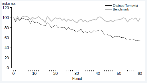
15.7 The limitations of traditional bilateral index formulae have motivated research by NSOs and academics into new methods for compiling price indexes from transactions data. Typically, multilateral index methods have been used in the spatial context to compare price levels across different geographic regions, however academics and NSOs are proposing they be used to make price comparisons across multiple (three or more) time periods. Multilateral methods have a number of advantages for temporal aggregation including:
- Using a census of products available in datasets;
- Weighting products at the product and elementary level by expenditure share;
- Price indexes that are free of 'chain drift'; and
- Reduced resources to produce indexes.
Methods for compiling transactions data
Background
15.8 Multilateral methods possess a number of desirable qualities, both theoretical and practical, to produce temporal price indexes from transactions data. The following details the practical and methodological decisions for aggregating transactions data in four sub-sections: aggregation structure, multilateral method, extension method and multilateral window length. This discussion returns to the framework established in the Information paper: Making Greater Use of Transactions Data to compile the Consumer Price Index (cat. no. 6401.0.60.003) which linked the ABS Data Quality Framework (DQF) to six main criteria for an NSO to evaluate different multilateral methods (Table 15.1).
| Consideration | Quality dimensions |
|---|---|
| Resources: does this method help facilitate more effective use of human and information resources? | Institutional Environment, Timeliness |
| Theoretical properties: what conceptual properties does the index method have, and how well do these align with the CPI purpose? | Accuracy |
| Transitivity: to what extent is the index transitive? | Accuracy, Coherence |
| Characteristicity: to what extent are price comparisons relevant to the time periods being compared? | Accuracy, Relevance |
| Flexibility: what scope is there to use or adapt the method for new statistical products or data sources? | Coherence, Institutional Environment |
| Interpretability: how easy is it to understand the method and the price movements it calculates? | Interpretability |
Product definition
15.9 The definition of a homogeneous product where the calculation of a unit value occurs remains largely consistent with previous practices in the CPI. The ABS defines products using product classifications provided by Australian proprietors known as the stock keeping unit (SKU). The unit value is calculated using expenditure and quantity information across all stores from the same proprietor for each capital city in Australia (e.g. SKU ‘xxx’ from Company 1 for Sydney).
15.10 The unit value is calculated on a quarterly frequency to align with the publication frequency of the Australian CPI. The quarterly unit value is calculated using approximately 2.5 months of revenue and quantity data in order to meet the timeliness constraints for publication - this is consistent with current ABS and international practices. This calculation of quarterly unit values differs slightly with previous CPI practice, where unit values were derived at both monthly and quarterly frequencies. Research has shown that the unit value calculation should align with the publication frequency of the CPI (Diewert, Fox and de Haan 2015).
15.11 The calculation of the unit value should occur across products that are considered equivalent from the perspective of a consumer. Research by other NSOs has shown that matched model multilateral indexes can have a downward bias if price increases are missed when the same item is ‘relaunched’ using a different product identifier (Chessa 2016). The issue of relaunches is a known problem when identifying products using barcodes for certain commodities, while the choice of a broader product definition such as SKU (which is an aggregation of multiple barcodes) should mitigate this problem. The ABS will continue to monitor the suitability of defining products using the SKU.
Elementary aggregation
15.12 In order to maximise the use of transactions data using multilateral methods, the ABS has modified the aggregation structure below the published (EC) level. Figure 15.2 details the aggregation structure implemented in the CPI, which uses respondent classes as elementary aggregates (EAs) when these are available from transactions datasets. The direct Törnqvist index formula is used to aggregate respondent EAs together to compile ‘Respondent x EC’ price indexes in order to capture changes in consumer expenditure patterns overtime. ‘Respondent x EC’ indexes are weighted by expenditure (market) share using the Lowe Index formula, with weights being reviewed on an annual basis using both transactions and other data sources.
Figure 15.2 Aggregation structure for transactions data ECs
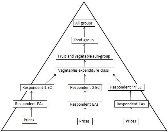
This diagram includes a pyramid outlining the aggregation structure for transactions data expenditure classes.
This begins at the base of the pyramid with prices. There are three streams which prices is at the base of. Each of the three streams flows up from prices to respondent elementary aggregates.
The first stream flows up from respondent elementary aggregates to respondent 1 expenditure class. The middle stream flows up from respondent elementary aggregates to respondent 2 expenditure class. The final stream flows up from respondent elementary aggregates to respondent ‘n’ expenditure class.
All three streams flow up from respondent 1, 2, and ‘n’ expenditure classes into vegetables expenditure class. This flows up to fruit and vegetable sub-group, which flows up to food group, and finally to all groups. All groups is the top of the pyramid.
15.13 The index structure described in Figure 15.2 includes contributions from transactions data respondents only. The 28 ECs that have this index structure are provided below in Table 15.2. The motivation to compile these ECs using transactions data only is based on evidence of high expenditure (market) share, as well as the resources required to maintain a high quality non-transactions data index component.
| EC |
|---|
| Beef and veal |
| Bread |
| Breakfast cereals |
| Cakes and biscuits |
| Cheese |
| Cleaning and maintenance products |
| Coffee, tea and cocoa |
| Eggs |
| Fish and other seafood |
| Food additives and condiments |
| Fruit |
| Ice cream and other dairy products |
| Jams, honey and spreads |
| Lamb and goat |
| Milk |
| Oils and fats |
| Other cereal products |
| Other food products n.e.c. |
| Other meats |
| Other non-durable household products |
| Personal care products |
| Pets and related products |
| Pork |
| Poultry |
| Snacks and confectionery |
| Tobacco |
| Vegetables |
| Water, soft drinks and juices |
Multilateral method
15.14 In recent years there has been an increase in the range of multilateral methods proposed for use in CPI aggregation when using transactions data. The Information paper: Making Greater Use of Transactions Data to compile the Consumer Price Index (cat. no. 6401.0.60.003) outlines research by the ABS into four multilateral methods considered for implementation into the Australian CPI(footnote 1) . These methods were:
- Weighted Time Product Dummy (TPD)
- Geary-Khamis (GK)
- Quality adjusted unit value using TPD (QAUV_TPD)
- Gini, Eltetö, Köves and Szulc (GEKS)-Törnqvist²
15.15 Testing the different multilateral methods in practice, the ABS found little difference in the empirical results generated from each different multilateral method. Comparing the different methods to the framework described in Table 15.1, the ABS preferred method for compiling price indexes using transactions data is the GEKS-Törnqvist. The two main criteria that differentiate the GEKS-Törnqvist from the other multilateral methods are its theoretical properties (economic approach to index numbers) and interpretability (based on bilateral index number theory). To remedy the sensitivity of the GEKS-Törnqvist to products with atypical prices and small quantities (clearance prices), the ABS uses filters to remove these products from index compilation. The exclusion of products at clearance prices is consistent with current practices adopted in the CPI.
15.16 The GEKS-Törnqvist method takes the geometric mean of the ratios of all bilateral Törnqvist indexes (calculated using the same index number formula) between a number of entities. For spatial indexes these entities are generally countries, while for price comparisons across time, the entities are time periods.
15.17 The bilateral index formula chosen for the Australian CPI is the Törnqvist index which can be expressed as:
\(P^{0,t}_{T}=\prod ^n_\limits {i=0}\Bigg[\frac{p^t_i}{p^0_i}\Bigg]^{\frac{s^t_i+s^0_i}{2}} \space \space \space \space \space (15.1)\)
where,
\(P^{0,t}_{T} = \) Törnqvist index between periods \(0\) and \(t\)
\(p^t_i =\) price of item \(i\) in period \(t\)
\(p^0_i=\) price of item \(i\) in period \(0\)
\({\frac{s^t_i+s^0_i}{2}}=\) average expenditure share of item \(i\) across periods \(0\) and \(t\)
15.18 The GEKS-Törnqvist is calculated as the geometric mean of the ratios of all matched-model Törnqvist bilateral indexes ( \(p^{l,0}\) and \(p^{l,t}\)) where each period is taken in turn as the base (de Haan 2015). The GEKS-Törnqvist method can be expressed as:
\(p_{GEKS}^{0,t}=\prod^T_\limits {l=0}\big[\frac{p^{l,t}}{p^{l,0}} \big] ^{\frac{1}{T+1}} \space \space \space \space \space (15.2)\)
\(P^{0,t}_{GEKS}=\) \(GEKS\) index between periods \(0\) and \(t\)
\(p^{l,0}=\) Törnqvist index between periods \(l\) and \(0\)
\(p^{l,t}=\) Törnqvist index between periods \(l\) and \(t\)
15.19 An example of calculating the GEKS-Törnqvist index across a three period multilateral window is provided below in Figure 15.3. Each row in the figure (or ratio term in the brackets) uses a Törnqvist index to measure price change between periods \(0\) and \(1\), where the base period changes for each row (ratio) whilst the comparison period remains constant. The GEKS then takes the geometric average of these three measures of price change between periods \(0\) and \(1\).
Figure 15.3: Example of GEKS-Tornqvist index
This image show the GEKS-Törnqvist index across a three period multilateral window. Each row in the figure (or ratio term in the brackets) uses a Törnqvist index to measure price change between periods 0 and 1, where the base period changes for each row (ratio) whilst the comparison period remains constant. The GEKS then takes the geometric average of these three measures of price change between periods 0 and 1.
Extension method
15.20 When multilateral methods are used to produce a temporal index, each bilateral price comparison depends on prices observed in other periods of the multilateral comparison window. As a result, incorporating a new period into the multilateral comparison window may revise previous price indexes, which is unacceptable for CPI purposes. To resolve this, researchers and NSOs have developed methods for using the latest multilateral index incorporating the latest data to update the published index series.
15.21 The ABS has considered a range of methods for extending the time series. These can be characterised into the following two groups³:
- The direct (annual) extension: method proposed by Chessa (2016). This involves extending the multilateral estimation window from some (annually) fixed base period as each new period becomes available, and using the price change between the base period and the new period to extend the series
- Rolling window methods inspired by Ivancic, Diewert and Fox (2011), which all involve calculating a new multilateral index using a window of fixed length as each new period becomes available. Having chosen some splice period common to the current and previous windows, the series is extended using the ratio of the price change between the splice period and the current period (using the current window) and the price change between the splice period and the previous period (using the previous window). Choosing the splice period to be the previous period yields a movement splice (Ivancic, Diewert and Fox 2011); choosing the start of the current window yields a window splice (Krsinich 2016); choosing the midpoint of the current window yields a half splice (de Haan 2015). Algebraically, the published index movement from the previous period (t -1) to the current period (t) can be expressed as:
\(p^{t-1,t}=\frac{p^{s,t}_M(current)}{p^{s,t-1}_M(previous)}\space \space \space \space \space (15.3)\)
where:
\(p^{s,t}_M(current)=\) price movement between the splice period \(s\) and \(t\) based on the current multilateral
\(p^{s,t-1}_M(previous)=\) price movement between \(s\) and \(t-1\) based on the previous multilateral window
15.22 While each of the rolling window methods above uses one specific splice period, Diewert and Fox (2017) have endorsed a mean splice rolling window method - initially proposed by Ivancic, Diewert and Fox (2011) - which involves extending the index using the geometric mean of the indexes produced from all possible choices of splice period. Using the notation above, the mean splice extension can be expressed algebraically as:
\(p^{t-1,t}=\prod ^{t-1}_ \limits {s=t-T}\Bigg(\frac{p^{s,t}_M(current)}{p^{s,t-1}_M(previous)}\Bigg)^\frac{1}{T} \space \space \space \space \space (15.4)\)
where the multilateral window length is \(T+1\) periods, so the current and previous periods overlap between \(t-T\) and \(t-1\).
15.23 The ABS has chosen the mean splice motivated by the following factors:
- Conceptually, it seems more natural to make the results independent of the choice of splice period by using all the periods they have in common, rather than choosing a single splice period.
- Empirically, the mean splice appears more robust - while the half splice mitigates systematic quality adjustment bias, choosing an alternative splice period close to the midpoint can give quite different results.
15.24 An example of the mean splice is provided below for a rolling window (length of five periods), where the price movement between periods four and five is estimated by taking the geometric mean of all ratios of GEKS indexes where each common splice period between window one and window two is taken in turn as the base (i.e. one, two, three and four). It can be shown that the mean splice effectively makes a small implicit revision to price movements early in the current window and a large implicit revision to price movements later in the current window. This mitigates the effect of both new and disappearing products, similar to the half splice.
Figure 15.4: Mean splice across rolling multilateral window
This image provides and example of the mean splice for a rolling window (length of five periods), where the price movement between periods four and five is estimated by taking the geometric mean of all ratios of GEKS indexes where each common splice period between window one and window two is taken in turn as the base (i.e. one, two, three and four). It shows that the mean splice effectively makes a small implicit revision to price movements early in the current window and a large implicit revision to price movements later in the current window. This mitigates the effect of both new and disappearing products, similar to the half splice.
Multilateral window length
15.25 The decision to implement a multilateral method requires an NSO to specify the number of time periods used for price comparisons. Most research involving rolling window approaches has recommended a minimum of one year and one period (i.e. five quarters, 13 months) to account for products seasonal availability, though there is currently no consensus on the optimal length of the multilateral window.
15.26 The choice of multilateral window length is a trade-off between two criteria - characteristicity and transitivity. If the multilateral window is too long, then the index could suffer from a loss of characteristicity where price change in the past may disproportionally impact recent inflation estimates. If the multilateral window is too short, the index may suffer from the ‘chain drift’ problem. Empirical testing of different window sizes is necessary to assist with this decision.
15.27 The Information paper: Making Greater Use of Transactions Data to compile the Consumer Price Index (cat. no. 6401.0.60.003) presented results that used a window size of two years and one period (i.e. nine quarters) as the preferred window length - this was based on empirically testing various estimation windows compared to each other (as well as their proximity to different ‘full’ reference price series). Empirical testing by the ABS showed that varying the length of the estimation window generally made little difference to the price series generated. The multilateral window length is two years and one period.
Consultation and future direction
15.28 The ABS undertook broad consultation regarding the implementation of multilateral methods to compile the Australian CPI. This commenced with the release of the Information paper: Making Greater Use of Transactions Data to compile the Consumer Price Index (cat. no. 6401.0.60.003), published 29 November 2016. Following this paper, the ABS sought user and stakeholder input to resolve the outstanding methodological challenges.
15.29 The ABS has collaborated with international experts and NSOs to resolve outstanding methodological issues. Additionally, the ABS conducted bilateral and multilateral consultations with key stakeholders, including: the Reserve Bank of Australia; the Treasury; Department of Social Services; Department of Finance; Department of Prime Minister and Cabinet; and State Treasuries. In all instances, experts, NSOs and stakeholders were supportive of maximising the use of transactions data to compile the CPI using multilateral methods.
15.30 The ABS will continue to monitor methodological developments in the use of transactions data to compile price indexes, as well as continue to conduct research into remaining practical issues including text mining, hedonics indexes, automated text mapping and the use of multilateral methods for aggregating prices ‘web scraped’ from online.
References
Australian Bureau of Statistics (ABS) 2016. Making Greater use of Transactions Data to Compile the Consumer Price Index. cat. no. 6401.0.60.003. ABS, Canberra.
Chessa, A. G. 2016. A new methodology for processing scanner data in the Dutch CPI. Eurostat review of National Accounts and Macroecnomic Indicators, 1, 49-70.
Diewert, E. W. 1995. Axiomatic and Economic Approaches to Elementary Price Indexes. Discussion Paper No. 95-01; Department of Economics, University of British Columbia.
Diewert, E. W., Fox, K. J. & de Haan, J. 2016. A newly identified source of potential CPI bias: Weekly versus monthly unit value price indexes. Economics Letters, 141, 169-172.
Diewert, E.W. & Fox, K.J. 2017. Substitution Bias in Multilateral Methods for CPI Construction using Scanner Data. Discussion Paper No. 17-02; Vancouver School of Economics, University of British Columbia.
de Haan, J. 2015. A Framework for Large Scale Use of Scanner Data in the Dutch CPI. Paper presented at the fourteenth Ottawa Group meeting. Tokyo, Japan.
de Haan, J. and van der Grient, H. 2011, Eliminating Chain Drift in Price Indexes Based on Scanner Data, Journal of Econometrics 161, 36-46.
International Labour Organization (ILO) 2004. Consumer Price Index Manual: Theory and practice, International Labour Office, Geneva.
Ivancic, L., Fox, K. J. & Diewert, E. W. 2011. Scanner data, time aggregation and the construction of price indexes. Journal of Econometrics, 161, 24-35.
Footnotes
Appendix 1 - CPI weighting pattern
| Percentage contribution to the All groups CPI | |||||
|---|---|---|---|---|---|
| Group, Sub-group, Expenditure class | % | % | % | ||
| FOOD AND NON-ALCOHOLIC BEVERAGES | 15.76 | ||||
| Bread and cereal products | 1.43 | ||||
| Bread | 0.53 | ||||
| Cakes and biscuits | 0.62 | ||||
| Breakfast cereals | 0.12 | ||||
| Other cereal products | 0.16 | ||||
| Meat and seafoods | 2.14 | ||||
| Beef and veal | 0.46 | ||||
| Pork | 0.29 | ||||
| Lamb and goat | 0.22 | ||||
| Poultry | 0.42 | ||||
| Other meats | 0.36 | ||||
| Fish and other seafood | 0.39 | ||||
| Dairy and related products | 0.96 | ||||
| Milk | 0.35 | ||||
| Cheese | 0.29 | ||||
| Ice cream and other dairy products | 0.32 | ||||
| Fruit and vegetables | 2.23 | ||||
| Fruit | 1.04 | ||||
| Vegetables | 1.19 | ||||
| Food products n.e.c. | 2.11 | ||||
| Eggs | 0.12 | ||||
| Jams, honey and spreads | 0.13 | ||||
| Food additives and condiments | 0.28 | ||||
| Oils and fats | 0.18 | ||||
| Snacks and confectionery | 0.88 | ||||
| Other food products n.e.c. | 0.52 | ||||
| Non-alcoholic beverages | 0.97 | ||||
| Coffee, tea and cocoa | 0.21 | ||||
| Waters, soft drinks and juices | 0.76 | ||||
| Meals out and take away foods | 5.92 | ||||
| Restaurant meals | 3.32 | ||||
| Take away and fast foods | 2.60 | ||||
| ALCOHOL AND TOBACCO | 7.36 | ||||
| Alcoholic beverages | 4.54 | ||||
| Spirits | 0.85 | ||||
| Wine | 1.74 | ||||
| Beer | 1.95 | ||||
| Tobacco | 2.82 | ||||
| Tobacco | 2.82 | ||||
| CLOTHING AND FOOTWEAR | 3.32 | ||||
| Garments | 2.03 | ||||
| Garments for men | 0.55 | ||||
| Garments for women | 1.15 | ||||
| Garments for infants and children | 0.33 | ||||
| Footwear | 0.50 | ||||
| Footwear for men | 0.13 | ||||
| Footwear for women | 0.30 | ||||
| Footwear for infants and children | 0.07 | ||||
| Accessories and clothing services | 0.79 | ||||
| Accessories | 0.67 | ||||
| Cleaning, repair and hire of clothing and footwear | 0.12 | ||||
| HOUSING | 23.19 | ||||
| Rents | 7.10 | ||||
| Rents | 7.10 | ||||
| New dwelling purchase by owner-occupiers | 8.05 | ||||
| New dwelling purchase by owner-occupiers | 8.05 | ||||
| Other housing | 3.55 | ||||
| Maintenance and repair of the dwelling | 2.05 | ||||
| Property rates and charges | 1.50 | ||||
| Utilities | 4.49 | ||||
| Water and sewerage | 1.01 | ||||
| Electricity | 2.54 | ||||
| Gas and other household fuels | 0.94 | ||||
| FURNISHINGS, HOUSEHOLD EQUIPMENT AND SERVICES | 8.89 | ||||
| Furniture and furnishings | 1.62 | ||||
| Furniture | 1.32 | ||||
| Carpets and other floor coverings | 0.30 | ||||
| Household textiles | 0.44 | ||||
| Household textiles | 0.44 | ||||
| Household appliances, utensils and tools | 1.49 | ||||
| Major household appliances | 0.39 | ||||
| Small electric household appliances | 0.31 | ||||
| Glassware, tableware and household utensils | 0.42 | ||||
| Tools and equipment for house and garden | 0.37 | ||||
| Non-durable household products | 2.48 | ||||
| Cleaning and maintenance products | 0.24 | ||||
| Personal care products | 0.99 | ||||
| Other non-durable household products | 1.25 | ||||
| Domestic and household services | 2.86 | ||||
| Child care | 1.23 | ||||
| Hairdressing and personal grooming services | 0.92 | ||||
| Other household services | 0.71 | ||||
| HEALTH | 5.69 | ||||
| Medical products, appliances and equipment | 1.14 | ||||
| Pharmaceutical products | 1.00 | ||||
| Therapeutic appliances and equipment | 0.14 | ||||
| Medical, dental and hospital services | 4.55 | ||||
| Medical and hospital services | 4.00 | ||||
| Dental services | 0.55 | ||||
| TRANSPORT | 10.48 | ||||
| Private motoring | 9.76 | ||||
| Motor vehicles | 2.56 | ||||
| Spare parts and accessories for motor vehicles | 0.74 | ||||
| Automotive fuel | 3.24 | ||||
| Maintenance and repair of motor vehicles | 1.83 | ||||
| Other services in respect of motor vehicles | 1.39 | ||||
| Urban transport fares | 0.72 | ||||
| Urban transport fares | 0.72 | ||||
| COMMUNICATION | 2.57 | ||||
| Communication | 2.57 | ||||
| Postal services | 0.09 | ||||
| Telecommunication equipment and services | 2.48 | ||||
| RECREATION AND CULTURE | 12.60 | ||||
| Audio, visual and computing equipment and services | 1.83 | ||||
| Audio, visual and computing equipment | 1.12 | ||||
| Audio, visual and computing media and services | 0.71 | ||||
| Newspapers, books and stationery | 0.66 | ||||
| Books | 0.22 | ||||
| Newspapers, magazines and stationery | 0.44 | ||||
| Holiday travel and accommodation | 6.01 | ||||
| Domestic holiday travel and accommodation | 2.91 | ||||
| International holiday travel and accommodation | 3.10 | ||||
| Other recreation, sport and culture | 4.10 | ||||
| Equipment for sports, camping and open-air recreation | 0.57 | ||||
| Games, toys and hobbies | 0.72 | ||||
| Pets and related products | 0.43 | ||||
| Veterinary and other services for pets | 0.38 | ||||
| Sports participation | 0.96 | ||||
| Other recreational, sporting and cultural services | 1.04 | ||||
| EDUCATION | 4.27 | ||||
| Education | 4.27 | ||||
| Preschool and primary education | 0.93 | ||||
| Secondary education | 1.73 | ||||
| Tertiary education | 1.61 | ||||
| INSURANCE AND FINANCIAL SERVICES | 5.86 | ||||
| Insurance | 1.29 | ||||
| Insurance | 1.29 | ||||
| Financial services | 4.57 | ||||
| Deposit and loan facilities (direct charges) | 0.57 | ||||
| Other financial services | 4.00 | ||||
| ALL GROUPS CPI | 100.00 | 100.00 | 100.00 | ||
- Any discrepancies between totals and sums of components in this Appendix are due to rounding
Appendix 2 - Analytical series
Introduction
1 Each review of the Consumer Price Index, the ABS assesses the analytical requirements of its users and the current relevance of each special analytical series published. The following separate inflation series are currently published to assist users analyse the CPI:
- All groups CPI, seasonally adjusted;
- Underlying trend series, 'Trimmed mean' and 'Weighted median';
- International trade exposure series, Tradables component;
- International trade exposure series, Non-tradables component;
- All groups CPI, goods component;
- All groups CPI, services component;
- All groups CPI including Deposit and loan facilities (indirect charges);
- Market goods and services excluding 'volatile items';
- All groups CPI excluding a CPI group for each of the eleven CPI Groups;
- All groups CPI excluding Housing and insurance and financial services;
- All groups CPI excluding Medical and hospital services;
- All groups CPI excluding food and energy;
- All groups CPI excluding 'volatile items';
2 These analytical series are published in table 8 of Consumer Price Index, Australia (cat. no. 6401.0) and are compiled by taking subsets of the CPI basket. Each series and their composition are outlined below.
Goods and services
3 The ABS has classified expenditure classes as goods or services based on the majority of products in each category. In the CPI, 60 out of the 87 expenditure classes, accounting for approximately 53 per cent of the All groups CPI by weight, have been classified as goods. The remaining 27 expenditure classes, accounting for approximately 47 per cent of the All groups CPI by weight, have been classified as services.
International trade exposure
4 The CPI Tradables and Non-tradables series, collectively known as the International Trade Exposure series, measure the contribution of imported and domestic inflation to overall household inflation. Identifying the source of household inflation aides the understanding and forecasting of inflation; as well as supporting monetary and fiscal policy decisions.
5 The International Trade Exposure series classifies the CPI expenditure classes as either tradables or non-tradables by assessing the degree to which their prices are affected by domestic developments and international competition. The tradables and non-tradables series are available each quarter in table 8 of Consumer Price Index, Australia (cat. no. 6401.0).
6 Expenditure classes were defined as tradables firstly by assessing the level of imports and exports to Australian production. If exports or imports exceeded 10 per cent of Australian production, the expenditure class was classified, by default, as tradable. To determine the final classification, supplementary data were used to assess the appropriateness of each of the expenditure classes default classification. Following this, the contribution of domestic taxes and subsides to the price paid by consumers was analysed. Since taxes and subsidies are a domestic impact on inflation, these expenditure classes were classified as non-tradables where these make a large contribution to the price paid by consumers.
7 For further information see the feature article Review of the Consumer Price Index International Trade Exposure Series (cat. no. 6401.0).
8 The ABS released the tradables and non-tradables price indexes from the June quarter 1998 based on 1993-1994 and 1994-1995 Input-Output tables and related product correspondences. For the 15th series CPI, the tradable and non-tradable classification was based on the 2001-02 Input-Output data and related product correspondences. For the 16th series CPI, the 2006-07 Input-Output tables and related product correspondences were used and an optimal threshold of 10% was applied to determine whether an industry is exportable or importable . The 2013-14 Input-Output tables were used to update the classification in December quarter 2016.
9 More information is available in Australian National Accounts: Input-Output Tables (cat. no. 5209.0.55.001).
10 Table A2.1 shows which expenditure classes are classified as tradables and which are classified as non-tradables. In aggregate, 49 expenditure classes, which account for approximately 35 per cent of the CPI by weight, are classified as tradables. The remaining 38 expenditure classes, accounting for approximately 65 per cent of the CPI by weight, are classified as non-tradable.
Seasonally adjusted series
11 Seasonal adjustment helps the analysis of price movements as it estimates and then removes influences that are systematic and calendar related from a time series. The seasonal adjustment methodology used to produce analytical measures of underlying inflation was replaced with standard ABS seasonal adjustment methodology with the introduction of the 16th series CPI. This ensures that seasonally adjusted CPI data are consistent with other ABS data and results in more transparent and robust analytical series.
12 The following analytical series are published using the ABS seasonal adjustment methodology:
(i) All Groups CPI, seasonally adjusted: where seasonality has been identified at the weighted average of eight capital cities level. Seasonal adjustment factors are calculated using the history of price changes up to the current quarter CPI and are revised each quarter. The time series began with the December quarter 1986, with an index reference period of 2011-12 = 100.0
(ii) Group and expenditure class level price indexes (seasonally adjusted): comprises the subset of seasonally adjusted groups and expenditure classes at the weighted average of eight capital cities level. The time series began at different time periods, the earliest being the September quarter 1972, with an index reference period of 2011-12 = 100.0.
(iii) Trimmed mean and Weighted median: two measures of underlying inflation. In the 15th series, these measures were calculated using a seasonal adjustment methodology developed by the Reserve Bank of Australia (RBA)¹. The 16th series replaced this methodology with standard ABS seasonal adjustment methodology. These time series began with the June quarter 2002, with an index reference period of 2011-12 = 100.0.
(iv) Tradables and Non-tradables (seasonally adjusted): these series measure the contribution of imported and domestic inflation to overall household inflation at the weighted average of eight capital cities level. These time series began with the June quarter 1998, with an index reference period of 2011-12 = 100.0.
13 More information on the seasonal adjustment methodology is available in Information paper: Seasonal adjustment of Consumer Price Indexes, (cat. no. 6401.0.55.003).
14 At the introduction of the 17th series, 57 out of the 87 expenditure classes are classified as seasonal. A description of which series are currently seasonally adjusted is published in Appendix 1 of every December quarter issue of Consumer Price Index, Australia (cat. no. 6401.0), following the annual seasonal re-analysis. Table A2.1 lists the expenditure class that are seasonally adjusted, current at the December quarter 2017.
Market goods and services excluding 'volatile items'
15 Market items are those available on the open market. The volatile items are Fruit, Vegetables and Automotive fuel.
Deposit and loan facilities (indirect charges)
16 One of the outcomes of the 16th series review was to remove the indirectly measured component of the Deposit and loan facilities index from the headline CPI until such time that the methods and data sources are sufficiently robust for its reintroduction to the CPI. The analytical series, All groups CPI including Deposit and loan facilities (indirect charges) includes the All groups CPI plus the indirectly measured component of the Deposit and loan facilities index.
| International Trade Exposure | Seasonal | ||||||
|---|---|---|---|---|---|---|---|
| CPI expenditure classes | Goods | Services | Tradables | Non-tradables | Including current period | Not including current period | Market goods and services excluding 'volatiles' |
| Bread | y | y | y | ||||
| Cakes and biscuits | y | y | y | y | |||
| Breakfast cereals | y | y | y | y | |||
| Other cereal products | y | y | y | y | |||
| Beef and veal | y | y | y | y | |||
| Pork | y | y | y | y | |||
| Lamb and goat | y | y | y | y | |||
| Poultry | y | y | y | y | |||
| Other meats | y | y | y | y | |||
| Fish and other seafood | y | y | y | y | |||
| Milk | y | y | y | y | |||
| Cheese | y | y | y | ||||
| Ice cream and other dairy products | y | y | y | y | |||
| Fruit(c) | y | y | y | ||||
| Vegetables(c) | y | y | y | ||||
| Eggs | y | y | y | y | |||
| Jams, honey and spreads | y | y | y | ||||
| Food additives and condiments | y | y | y | y | |||
| Oils and fats | y | y | y | y | |||
| Snacks and confectionery | y | y | y | y | |||
| Other food products n.e.c. | y | y | y | y | |||
| Coffee, tea and cocoa | y | y | y | ||||
| Waters, soft drinks and juices | y | y | y | y | |||
| Restaurant meals | y | y | y | ||||
| Take away and fast foods | y | y | y | y | |||
| Spirits | y | y | y | ||||
| Wine | y | y | y | y | |||
| Beer | y | y | y | ||||
| Tobacco | y | y | y | y | |||
| Garments for men | y | y | y | y | |||
| Garments for women | y | y | y | y | |||
| Garments for infants and children | y | y | y | y | |||
| Footwear for men | y | y | y | y | |||
| Footwear for women | y | y | y | y | |||
| Footwear for infants and children | y | y | y | y | |||
| Accessories | y | y | y | y | |||
| Cleaning, repair and hire of clothing and footwear | y | y | y | y | |||
| Rents | y | y | y | y | |||
| New dwelling purchase by owner-occupiers | y | y | y | ||||
| Maintenance and repair of the dwelling | y | y | y | y | |||
| Property rates and charges | y | y | y | ||||
| Water and sewerage | y | y | y | ||||
| Electricity | y | y | y | ||||
| Gas and other household fuels | y | y | y | ||||
| Furniture | y | y | y | y | |||
| Carpets and other floor coverings | y | y | y | y | |||
| Household textiles | y | y | y | y | |||
| Major household appliances | y | y | y | y | |||
| Small electric household appliances | y | y | y | y | |||
| Glassware, tableware and household utensils | y | y | y | y | |||
| Tools and equipment for house and garden | y | y | y | y | |||
| Cleaning and maintenance products | y | y | y | ||||
| Personal care products | y | y | y | ||||
| Other non-durable household products | y | y | y | y | |||
| Child care | y | y | y | ||||
| Hairdressing and personal grooming services | y | y | y | ||||
| Other household services | y | y | y | ||||
| Pharmaceutical products | y | y | y | ||||
| Therapeutic appliances and equipment | y | y | |||||
| Medical and hospital services | y | y | y | ||||
| Dental services | y | y | y | ||||
| Motor vehicles | y | y | y | y | |||
| Spare parts and accessories for motor vehicles | y | y | y | y | |||
| Automotive fuel(c) | y | y | y | ||||
| Maintenance and repair of motor vehicles | y | y | y | y | |||
| Other services in respect of motor vehicles | y | y | y | ||||
| Urban transport fares | y | y | y | ||||
| Postal services | y | y | |||||
| Telecommunication equipment and services | y | y | y | ||||
| Audio, visual and computing equipment | y | y | y | y | |||
| Audio, visual and computing media and services | y | y | y | ||||
| Books | y | y | y | y | |||
| Newspapers, magazines and stationery | y | y | y | y | |||
| Domestic holiday travel and accommodation | y | y | y | y | |||
| International holiday travel and accommodation | y | y | y | y | |||
| Equipment for sports, camping and open-air recreation | y | y | y | ||||
| Games, toys and hobbies | y | y | y | y | |||
| Pets and related products | y | y | y | y | |||
| Veterinary and other services for pets | y | y | y | y | |||
| Sports participation | y | y | y | y | |||
| Other recreational, sporting and cultural services | y | y | y | y | |||
| Preschool and primary education | y | y | y | ||||
| Secondary education | y | y | y | ||||
| Tertiary education | y | y | y | ||||
| Insurance | y | y | y | y | |||
| Deposit and loan facilities (direct charges) | y | y | y | ||||
| Other financial services | y | y | y | ||||
- As at December quarter 2018
- y = yes
- volatile items
Footnotes
Appendix 3 - Financial services in the consumer price index
Introduction
1 The purpose of this appendix is to outline the measurement of financial services in the Australian Consumer Price Index (CPI). The appendix also discusses research directions and future developments in the measurement of financial services.
2 The decision to introduce a price index for financial services into the Australian CPI was an outcome of the 13th series review of the Australian CPI conducted in 1997. Consistent with the objective of the CPI as a measure of price inflation for the household sector as a whole, the price index covered all those services acquired by households in relation to the acquisition, holding and disposal of financial and real assets. The index measured the price change for some of the most significant financial services acquired by households - deposit and loan facilities provided by financial institutions and services associated with the acquisition and disposal of real estate.
3 Financial services were introduced into the 15th series Australian CPI in the September quarter 2005 issue following developmental work described in the Information Paper: Experimental Price Indexes for Financial Services, 1998 to 2003 (cat. no. 6413.0), which was released in July 2004. The experimental series was published quarterly in Experimental Price Indexes for Financial Services (cat. no. 6413.0.55.001) up until June quarter 2005.
4 The ABS is the only national statistical agency that has constructed such a comprehensive measure of price change for financial services for use in their CPI. Financial services price indexes were published for two components: ‘Deposit and loan facilities’ and ‘Other financial services’.
- ‘Deposit and loan facilities’ included indirect charges recouped by intermediaries (prices derived from interest rate margins) and direct charges levied for services including withdrawals, maintenance of accounts and arranging loans.
- ‘Other financial services’ were restricted to services provided by stockbrokers and real estate agencies, legal and conveyancing fees and taxes levied on relevant transactions.
5 Volatility in the Deposit and loans facilities index during the Global Financial Crisis (GFC) prompted concerns from users about the quality, interpretability and transparency of the index. There was strong stakeholder support for a detailed reassessment of the Deposit and loan facilities index. These concerns led to significant analysis of the indirect charges component of the Deposit and loans facilities in close consultation with end users and data providers as part of the 16th series review of the Australian CPI. The review concluded that conceptually both direct and indirect charges for Deposit and loan facilities should be included in the CPI. However, the GFC has demonstrated that the internationally recognised methodology employed by the ABS to calculate the indirect charges component of the CPI, was not sufficiently robust to produce a high quality estimate of price change under all economic circumstances. It also became apparent that, if the index is to deliver accurate results in all economic conditions, very detailed, high quality data are required from reporting financial institutions. To ensure the high quality of the financial services component of the CPI the indirectly measured component of the Deposit and loan facilities index was removed from the headline CPI from the commencement of the 16th series CPI in the September quarter 2011.
6 Further information is contained in Information Paper: Outcome of the 16th Series Australian Consumer Price Index Review, Australia (cat. no. 6469.0).
Deposit and loan facilities in the CPI
Background
7 The Deposit and loan facilities index in the 15th series CPI measured changes in the price of banking services provided to households. Households pay for these banking services in two ways, directly and indirectly. Charges are paid for items including regular monthly fees, transaction fees such as automated teller machine (ATM) access fees, and the arrangement or cessation of products such as loans. These are termed direct charges. Banks also earn income by lending funds at a higher rate of interest than they pay on deposits. The difference can be described as 'interest rate margins' which are termed indirect charges. These are referred to in economic accounts and statistical literature as financial intermediation services indirectly measured (FISIM).
8 The ABS believes that conceptually both indirect charges and direct charges should be included in the headline CPI as they are real payments for services consumed by households. Financial institutions often substitute between direct and indirect forms of charging. Therefore a comprehensive measure of price change for deposit and loan facilities should include both the direct and indirect components. This conceptual view was widely supported by users in submissions and consultations as part of the 16th series review of the Australian CPI undertaken in 2010. Nonetheless there were key concerns around the predictability, interpretability, data quality and lack of international methodological consensus of the indirect fee measure (such as the treatment of default risk and term risk). The financial market volatility of the GFC, characterised by sudden movements in market and policy interest rates, heightened these concerns to the point that the quality of this component of the measure of financial services in the CPI was brought into question.
9 Following extensive stakeholder consultation the ABS decided to change the measurement of financial services in the CPI in the 16th series CPI, from the September quarter 2011. The changes were as follows:
- the indirectly measured component of the Deposit and loan facilities index was removed from the headline CPI; and
- the Deposit and loan facilities index comprised direct fees and charges only and was renamed 'Deposit and loan facilities (direct charges)'.
10 The CPI expenditure class 'Deposit and loan facilities (direct charges)' begins with an index reference period of 2011-12 = 100.0 and measures the change in prices of direct charges only. To assist users in understanding the impact on inflation of both direct and indirect charges, the ABS also publishes an analytical series, ‘All groups CPI including Deposit and loan facilities (indirect charges)’, which is published on a quarterly basis.
Direct charges - expenditure weights
11 Along with the decision to publish ‘Deposit and loan facilities (direct charges)’, the ABS reviewed the methodologies for calculating the expenditure weight and price movements for this direct charge component. For most financial services expenditure cannot be determined from the ABS Household Expenditure Survey (HES) as it is either not directly observed or the HES does not capture the transactions in sufficient volumes or detail.
12 As such, expenditure on Deposit and loan facilities (direct charges) is determined through the use of administrative data sets (obtained from financial institutions and government reporting agencies) of financial institution fees and charges for Australian households. For the 17th series CPI the capital city level estimates were imputed by reference to data from the 2015-16 HES and revalued to the price reference period (September quarter 2017).
Direct charges - price change
13 The pricing schedules that determine the amounts payable as explicit fees are generally not linear in nature and tend to incorporate some form of step function. In other words, rather than setting a single price per transaction, it is often the case that fees for certain types of transactions are only incurred after some threshold is breached (for example, after four transactions in a month or when account balances fall below some level). Furthermore, financial institutions often bundle products together, with the price paid for particular banking products (such as home loans, credit cards and transaction accounts) depending on the bundling arrangements.
14 To measure the price change faced by households in the 15th series CPI, the ABS selected a sample of customer accounts which represented consumer behaviour and applied the fee schedule for the relevant banking products in the period. However, it was not possible to update the sample of customer accounts as frequently as new products were introduced, leading to the sample becoming out of date.
15 To ensure the measurement of fees is relevant, the ABS modified the measurement of price change from the 16th series CPI in the September quarter 2011. The measurement of fees and charges has changed from the sample of customer accounts approach to a direct collection of a sample of fees and charges on banking products and services from financial institutions. This practice has continued for the 17th series introduced in the December quarter 2017.
16 The fee collection includes charges for ATM transactions, credit card annual fees, foreign currency conversion fees, account keeping fees, exception fees, loan servicing fees, package fees and others. Each month the price, terms and conditions for each banking product are observed. The sampled fees are grouped by type of product or service (e.g. credit cards, housing loans) and applied an appropriate weight to ensure representative derivation of price change for each product group. The product groups are then aggregated to provide a measure of average price change representing all direct fees and charges levied on consumers for banking products and services. In the case of fees levied as a percentage of a value, such as foreign currency conversion fees, the percentage fee is applied to a sample of dollar values representing real average transactions. To preserve the quantities underpinning the values of the account transactions in the price reference period, the transactions used to derive the dollar values of the fees are indexed each period using a four quarter moving average of the All groups CPI. This is consistent with the fixed basket approach to the CPI.
17 The sample of fees and charges are updated regularly to reflect any changes in consumer behaviour and financial institution fee regimes. The direct collection of fees and charges on a sample of popular banking products and services is consistent with methods employed by other national statistical organisations.
18 For each selected institution, the individual fees are combined using the Relative of Average Prices (RAP) method within a product type. Expenditure data described in the section above is then used to aggregate up to the published level. See Price index theory of this manual for more information on calculation methods.
Indirect charges - expenditure weights
19 The expenditure weight for Deposit and loan facilities (indirect charges), which is included in the analytical series, ‘All groups CPI including Deposit and loan facilities (indirect charges)’ is estimated from the dollar margins on each product provided by financial institutions. Information on calculating reference rates, product yields and dollar margins is included below in the section on measuring price change.
20 For all those products identified as being consumer products (as distinct from those used by businesses), the total receipts from households are combined to derive the total household margin by institution. These margins for each sampled institution are then applied to aggregate balances for all deposit taking institutions (sourced from the Australian Prudential Regulation Authority (APRA)) to derive a national estimate. For the 17th series CPI the capital city level estimates were imputed by reference to data from the 2015-16 HES and revalued to the price reference period (September quarter 2017).
Indirect charges - price change
21 The methodology to calculate the indirect banking service charge in the analytical series ‘All groups CPI including Deposit and loan facilities (indirect charges)’ is broadly consistent with the approach used to calculate this component of the Deposit and loan facilities index in the 15th series of the CPI. Improvements in the price calculation process for indirect banking service charges were made as part of the 16th series review, including sourcing a comprehensive dataset of consumer banking products from selected financial institutions and increased product level detail. Regular re-weighting of banking products was also introduced to ensure the relevance of the sample is maintained. The following sections describe these improvements in further detail.
22 The ABS obtains average monthly balances and interest flows data from selected financial institutions for each of their consumer products to calculate the indirect banking service charge. A separate reference rate of interest is calculated for each institution as the mid-point of weighted average borrowing and lending rates. The reference rate represents a ‘service free rate’ and is used as a means of partitioning the value of the financial intermediation service between borrowers and lenders. It is important to recognise that this mid-point reference rate is not intended to approximate a financial institution's cost of funds.
23 For each institution, the sampled consumer banking products are assigned to major product categories. The product yield for each product is determined by dividing the annualised interest by the average product balance. The interest margin for consumer products is calculated from the difference between the product yield and the reference rate. For deposit accounts the interest margin is the reference rate less the product yield, for loan accounts it is the product yield less the reference rate.
24 Because percentages (such as margin rates) are not prices, the latest period margin rates are applied to some monetary amount in order to compute the current period prices (the dollar value of the margins). Price reference period balances on the sample of products are used for this purpose to derive the dollar value of the margins. To preserve the quantities underpinning the values of the account balances in the price reference period, the balances used to derive the dollar values of the margins are indexed each quarter using a four quarter moving average of the All groups CPI. This is consistent with the fixed basket approach to the CPI.
25 The indirect component of the Deposit and loan facilities index is calculated by aggregating the dollar margins from the individual products and product groups, giving a weighted total margin paid for both deposit and loans. The price index is constructed by comparing the change over time in these total margins. It is important to note that prices on any single product are affected by changes in both the yield on that product, and the institution specific reference rate. Disaggregation of the balances (stocks) and interest (flows) to the individual product level improves the accuracy of the product categorisation and the robustness of the final aggregation of the index.
26 To minimise the effect of any short-term accounting anomalies the ABS constructs three month moving averages of the monthly balances and interest flows and derives the required product yields, reference rates and margin rates from the smoothed data. In addition, data are provided by the sampled financial institutions on a one month lag basis.
Developments in the measurement of deposit and loan facilities (indirect charges)
27 A major focus of the 16th series review of the Australian CPI was a research effort into issues surrounding the measurement of the indirect charges component of the Deposit and loan facilities index in the 15th series CPI. The review recommended the Deposit and loan facilities index comprising direct and indirect charges be re-introduced into the headline CPI when the ABS is satisfied that the methodology and data are sufficiently robust to produce high quality estimates, under all economic conditions. The ABS had planned to reintroduce the FISIM (indirect charges) series within the CPI in time for the introduction of the 17th series CPI. However, while the ABS has engaged internationally in attempts to resolve the methodological challenges associated with its measurement, many of the challenges identified as part of the 16th series remain. As a result, the ABS has not reintroduced FISIM into the headline CPI for the 17th series. The ABS will continue to produce the analytical series 'All groups CPI including Deposit and loan facilities (indirect charges)', and work with our international partners in the resolution of measurement challenges.
Other financial services in the CPI
Background
28 The Other financial services index was introduced into the 15th series CPI in 2005. Other financial services covers the cost of those services acquired by households in selling or buying major assets such as real estate and equities (shares) and any government charges on property transfers. Other financial services in the CPI consists of five components; taxes on property transfers (stamp duty), stockbroking services, legal and conveyancing services, accounting services and real estate agent services. The inclusion of superannuation and life insurance service charges are being considered as part of an ongoing research and consultation effort.
Other financial services - expenditure weights
29 The expenditure weight for the taxes on property transfers (stamp duty) measure is derived from the publication Taxation Revenue, Australia (cat. no. 5506.0), and data supplied by the State and Territory Revenue Offices. The annual Taxation Revenue publication contains statistics of taxation revenue collected by all levels of government in Australia. The expenditure weight for stockbroking services is obtained from National Accounts Household Final Consumption Expenditure (HFCE) data on stockbroking services by state. The expenditure weight for legal and conveyancing services, as well as real estate agent services are derived from National Accounts Private Gross fixed capital formation (GFCF) ownership transfer costs series. Expenditure weights for accounting services are derived from HES data.
Other financial services - price change
30 Data used in the pricing of Other financial services are collected from a range of providers and administrative datasets, including from real estate agents, accounting and legal firms, and state and territory revenue offices.
31 The measurement of real estate agent commission fees is not directly observed each period as the service provided varies from property to property and agents typically quote their fees as some percentage of the sale price of the property. In common with other items, where charges are determined as a 'margin', this needs to be converted to a 'dollar' price. If the percentage margin is known, the agents' price for any given transaction is computed by multiplying the sale price of the property by the percentage margin. The ABS conducts a quarterly survey of real estate agents in each capital city. For each transaction, the agent reports the sale price of the property and the total dollar amount of commission charged by the agent. The ABS uses ordinary least squares regression techniques to estimate a relationship between property values and commission rates.
32 The functional form used to fit the survey data and estimate this relationship was updated for the 16th series CPI to include location of a property sale as an explanatory variable. The sample of property sale transactions is updated biennially, and from the 16th series CPI includes residential units as well as detached houses. The price reference period sample prices are indexed using a four term moving average of the CPI to keep the quantity of service fixed. For the CPI, the quantity refers to a transaction value of investing in real estate and is measured in terms of forgone consumption.
33 The functional form used in the 17th series CPI remains the same as the functional form used in the 16th series CPI. The commission rate is modelled as a function of the inverse of the sale price and a location specific variable to account for differences in geographic areas.
\(Commission_{t}=\beta_{0}+\frac{\beta_{1}}{sale\ price}+\sum_\limits {i=1}^{N} \delta_{i} C_{i}+\varepsilon_{i}\)
Where:
\(Commission\) is the commission rate
\(sale\ price\) is the sale price of the property
\(\beta_{0}\) is a universal constant
\(\beta_{1}\) is a slope parameter to be estimated
\(\delta_{i}\) is a constant for each location (\(i\) = 1,2,3,...)
\( C_{i}\) represents each location (\(i\) = 1,2,3,...)
\(\varepsilon\) is the error term
34 The calculation of price change for the taxes on transfers component is done by applying the duty rates for each state and territory to a sample of property sale transactions for the respective state and territory. The price reference period sample of property prices are indexed using a four term moving average of the CPI to keep the quantity of service fixed. Prices for accounting services are sourced from the Producer Price Indexes (PPI), while legal and conveyancing fees are sourced from the Wage Price Index (WPI). Stockbroking fees are not currently priced directly, but are imputed by the movement in accounting fees. Development of a price index for this component is in the future CPI work program.
Superannuation and life insurance services
35 Financial services provided in relation to superannuation and life insurance products are within the conceptual scope of a Consumer Price Index produced on an acquisitions basis. In accordance with the outcome of the 16th series review of the Australian CPI in December 2010, the ABS is researching the development of a superannuation and life insurance services index. Methodologies and data sources are being investigated for both the expenditure weight and price measurement of Superannuation and life insurance services in the CPI.
36 The complexity of the charging arrangements for services provided by life insurance offices and superannuation funds, and the industry itself, makes it difficult to create a robust and representative price measure. Superannuation contributions and life insurance premiums have three components: a savings component for the insurance/superannuation itself, an explicit service charge payable to the enterprise for arranging the insurance/superannuation and an implicit service charge payable to the enterprise for arranging the insurance/superannuation. The implicit service charge payable for facilitating life insurance and superannuation is an integral part of the gross premium and contribution, but in practice is difficult to separate and measure.
37 The ABS aims to introduce the superannuation and life insurance price series initially as an experimental series to allow examination of the behaviour and effect of the series on the headline CPI. The ABS would need to be satisfied that the methodology and data are sufficiently robust to produce high quality estimates over a sufficiently long time series and different economic conditions. The ABS will consult widely with key stakeholders and users of the CPI before reaching any such decision. The development of price indexes for superannuation and life insurance indexes will be assessed in the context of the overall CPI forward work program.
References
Australian Bureau of Statistics 2004, Information Paper: Experimental Price Indexes for Financial Services, 1998 to 2003, (cat. no. 6413.0), July 2004, ABS, Canberra.
Australian Bureau of Statistics, 2008, Consumer Price Index, Australia, (cat. no. 6401.0), June 2008, ABS, Canberra.
Australian Bureau of Statistics 2009, Australian Consumer Price Index: Concepts, Sources and Methods, (cat. no. 6461.0), December 2009, ABS, Canberra.
Australian Bureau of Statistics 2010, Information Paper: Outcome of the 16th Series Australian Consumer Price Index Review, (cat. no. 6469.0), December 2010, ABS, Canberra.
Cullen, D., Kluth, S.(2010), A progress report on ABS investigations into FISIM in National Accounts, Consumer Price Index and Balance of Payments. Paper presented at the ISWGNA Meeting of the FISIM Task Force March 2011. Available at http://unstats.un.org/unsd/nationalaccount/RAmeetings/TFMar2011/lod.asp.
Diewert, W.E, Fixler, D, Zieschang, K. (2011), The Measurement of Banking Services in the System of National Accounts. Paper presented at Ottawa Group Meeting 2011. Available at http://www.stats.govt.nz/ottawa-group-2011/agenda.aspx.
Schreyer, P. (2009), A General Equilibrium Asset Approach to the Measurement of Nominal and Real Bank Output: Comment, pp. 320-328 in Price Index Concepts and Measurement, W.E. Diewert, J. Greenlees and C. Hulten (eds.), Studies in Income and Wealth, Volume 70, Chicago: University of Chicago Press.
United Nations Statistics Division 2010 Terms of Reference for the Task Force on Financial Intermediation Services Indirectly Measured (FISIM). Available at http://unstats.un.org/unsd/nationalaccount/criList.asp.
Appendix 4 - ILO resolution concerning consumer price indices
Introduction
This appendix has been extracted from the website of the International Labour Organization (ILO). It reproduces the resolution concerning consumer price indices adopted by the Seventeenth International Conference of Labour Statisticians, 2003. The resolution can be found at
http://www.ilo.org/public/english/bureau/stat/download/res/cpi2.pdf.
It is also reproduced at annex 3 of the international Consumer Price Index Manual published by the ILO.
Resolution II
Resolution concerning consumer price indices
Preamble
The Seventeenth International Conference of Labour Statisticians,
Having been convened at Geneva by the Governing Body of the ILO and having met from 24 November to 3 December 2003,
Recalling the resolution adopted by the Fourteenth International Conference of Labour Statisticians concerning consumer price indices and recognizing the continuing validity of the basic principles recommended therein and, in particular, the fact that the consumer price index (CPI) is designed primarily to measure the changes over time in the general level of prices of goods and services that a reference population acquires, uses or pays for,
Recognizing the need to modify and broaden the existing standards in the light of recent methodological and computational developments to enhance the usefulness of the international standards in the provision of technical guidelines to all countries,
Recognizing the usefulness of such standards in enhancing the international comparability of the statistics,
Recognizing that the CPI is used for a wide variety of purposes and that governments should be encouraged to identify the (priority) purposes a CPI is to serve, to provide adequate resources for its compilation, and to guarantee the professional independence of its compilers,
Recognizing that the (priority) objectives and uses of CPI differ among countries and that, therefore, a single standard could not be applied universally,
Recognizing that the CPI needs to be credible to observers and users, both national and international, and that better understanding of the principles and procedures used to compile the index will enhance the users' confidence in the index,
Agrees that the principles and methods used in constructing a CPI should be based on the guidelines and methods that are generally accepted as constituting good statistical practices;
Adopts, this third day of December 2003, the following resolution which replaces the previous one adopted in 1987:
The nature and meaning of a consumer price index
1 The CPI is a current social and economic indicator that is constructed to measure changes over time in the general level of prices of consumer goods and services that households acquire, use or pay for consumption.
2 The index aims to measure the change in consumer prices over time. This may be done by measuring the cost of purchasing a fixed basket of consumer goods and services of constant quality and similar characteristics, with the products in the basket being selected to be representative of households' expenditure during a year or other specified period. Such an index is called a fixed-basket price index.
3 The index may also aim to measure the effects of price changes on the cost of achieving a constant standard of living (i.e. level of utility or welfare). This concept is called a cost-of-living index (COLI). A fixed basket price index, or another appropriate design, may be employed as an approximation to a COLI.
The uses of a consumer price index
4 The CPI is used for a wide variety of purposes, the two most common ones being: (i) to adjust wages as well as social security and other benefits to compensate, partly or completely, for changes in the cost of living or in consumer prices; and (ii) to provide an average measure of price inflation for the household sector as a whole, for use as a macro- economic indicator. CPI subindices are also used to deflate components of household final consumption expenditure in the national accounts and the value of retail sales to obtain estimates of changes in their volume.
5 CPIs are also used for other purposes, such as monitoring the overall rate of price inflation for all sectors of the economy, the adjustment of government fees and charges, the adjustment of payments in commercial contracts, and for formulating and assessing fiscal and monetary policies and trade and exchange rate policies. In these types of cases, the CPI is used as more appropriate measures do not exist at present, or because other characteristics of the CPI (e.g. high profile, wide acceptance, predictable publication schedule, etc.) are seen to outweigh any conceptual or technical deficiencies.
6 Given that the CPI may be used for many purposes, it is unlikely that one index can perform equally satisfactorily in all applications. It may therefore be appropriate to construct a number of alternative price indices for specific purposes, if the requirements of the users justify the extra expense. Each index should be properly defined and named to avoid confusion and a "headline" CPI measure should be explicitly identified.
7 Where only one index is compiled, it is the main use that should determine the type of index compiled, the range of goods and services covered, its geographic coverage, the households it relates to, as well as to the concept of price and the formula used. If there are several major uses, it is likely that compromises may have to be made with regard to how the CPI is constructed. Users should be informed of the compromises made and of the limitations of such an index.
Scope of the index
8 The scope of the index depends on the main use for which it is intended, and should be defined in terms of the type of households, geographic areas, and the categories of consumer goods and services acquired, used or paid for by the reference population.
9 If the primary use of the CPI is for adjusting money incomes, a relevant group of households, such as wage and salary earners, may be the appropriate target population. For this use, all consumption expenditures by these households, at home and abroad, may be covered. If the primary use of the CPI is to measure inflation in the domestic economy, it may be appropriate to cover consumption expenditures made within the country, rather than the expenditures of households resident within the country.
10 In general, the reference population for a national index should be defined very widely. If any income groups, types of households or particular geographic areas are excluded, for example, for cost or practical considerations, then this should be explicitly stated.
11 The geographic scope refers to the geographic coverage of price collection and of consumption expenditures of the reference population and both should be defined as widely as possible, and preferably consistently. If price collection is restricted to particular areas due to resource constraints, then this should be specified. The geographic coverage of the consumption expenditure may be defined either as covering consumption expenditure of the resident population (resident consumption) or consumption expenditure within the country (domestic consumption).
12 Significant differences in the expenditure patterns and/or price movements between specific population groups or regions may exist, and care should be taken to ensure that they are represented in the index. Separate indices for these population groups or regions may be computed if there is sufficient demand to justify the additional cost.
13 In accordance with its main purpose, the CPI should conceptually cover all types of consumer goods and services of significance to the reference population, without any omission of those that may not be legally available or may be considered socially undesirable. Where appropriate, special aggregates may be constructed to assist those users who may wish to exclude certain categories of goods or services for particular applications or for analysis. Whenever certain goods or services have been excluded from the index, this should be clearly documented.
14 Goods and services purchased for business purposes, expenditures on assets such as works of art, financial investment (as distinct from financial services), and payments of income taxes, social security contributions and fines are not considered to be consumer goods or services and should be excluded from the coverage of the index. Some countries regard expenditures on the purchase of houses entirely as a capital investment and, as such, exclude them from the index.
Acquisition, use or payment
15 In determining the scope of the index, the time of recording and valuation of consumption, it is important to consider whether the purposes for which the index is used are best satisfied by defining consumption in terms of "acquisition", "use", or "payment". (See Annex 1) The "acquisition" approach is often used when the primary purpose of the index is to serve as a macroeconomic indicator. The "payment" approach is often used when the primary purpose of the index is for the adjustment of compensation or income. Where the aim of the index is to measure changes in the cost of living, the "use" approach may be most suitable. The decision regarding the approach to follow for a particular group of products should in principle be based on the purpose of the index, as well as on the costs and the acceptability of the decision to the users who should be informed of the approach followed for different products. Because of the practical difficulties in uniformly defining consumption and estimating the flow of services provided by other durable goods in terms of "use", it may be necessary to adopt a mixed approach, e.g. "use" for owner-occupied housing and "acquisition" or "payments" basis for other consumer durables.
16 The differences between the three approaches are most pronounced in dealing with products for which the times of acquisition, use and payment do not coincide, such as owner-occupied housing, durable goods and products acquired on credit.
17 The most complex and important of the products mentioned above is owner-occupied housing. In most countries, a significant proportion of households are owner-occupiers of their housing, with the housing being characterized by a long useful life and a high purchase outlay (price). Under the "acquisition" approach, the value of the new dwellings acquired in the weights reference period may be used for deriving the weight (and the full price of the dwelling is included in the CPI at the time of acquisition, regardless of when the consumption is taking place). Under the "payment" approach, the weights reflect the amounts actually paid out for housing (and the prices enter the CPI in the period(s) when the prices are paid). Under the "use" approach the weights are based on the value of the flow of housing services consumed during the weights reference period estimated using an implicit or notional cost (and prices or estimated opportunity costs enter the CPI when the consumption is taking place).
18 Own-account consumption, remuneration in kind and/or goods and services provided without charge or subsidized by governments and non-profit institutions serving households may be important in some countries where the purpose of the index is best satisfied by defining consumption in terms of "use" or "acquisition" (under the payment approach these are out of scope). The inclusion of these products will require special valuation and pricing techniques.
Basket and weights
19 Decisions on the composition of the basket and the weights follow directly from the scope, as well as from the choice between the "acquisition", "use" or "payment" approaches.
20 Once defined, the expenditures that fall within the scope of the index should be grouped into similar categories in a hierarchical classification system, e.g. divisions/groups/classes, for compilation as well as analytical purposes. There should be consistency between the classification used for index compilation and the one used for household expenditure statistics. The CPI classification should meet the needs of users for special subindices. For the purposes of international comparisons, the classification should also be reconcilable with the most recent version of the UN Classification of Individual Consumption According to Purpose (COICOP), at least at its division level.(See Annex 4)
21 In order to facilitate the analysis and interpretation of the results of the index, it may be desirable to classify goods and services according to various supplementary classifications, e.g. source of origin, durability and seasonality. Calculation of the CPI by using various classifications should generate the same overall results as the original index.
22 The classification should also provide a framework for the allocation of expenditure weights. Expenditures at the lowest level of the classification system, expressed as a proportion of the total expenditure, determine the weights to be used at this level. When the weights are to remain fixed for several years, the objective should be to adopt weights that are representative of the contemporary household behaviour.
23 The two main sources for deriving the weights are the results from household expenditure surveys (HESs) and national accounts estimates on household consumption expenditure. The results from an HES are appropriate for an index defined to cover the consumption expenditures of reference population groups resident within the country, while national account estimates are suitable for an index defined to cover consumption expenditures within the country. The decision about what source or sources to use and how they should be used depends on the main purpose of the index and on the availability and quality of appropriate data.
24 The information from the main source (HESs or national accounts) should be supplemented with all other available information on the expenditure pattern. Sources of such information that can be used for disaggregating the expenditures are surveys of sales in retail outlets, point-of-purchase surveys, surveys of production, export and import data and administrative sources. Based on these data the weights for certain products may be further disaggregated by region and type of outlet. Where the data obtained from different sources relate to different periods, it is important to ensure, before weights are allocated, that expenditures are adjusted so that they have the same reference period.
25 Where the weight reference period differs significantly from the price reference period, the weights should be price updated to take account of price changes between the weights reference period and price reference period. Where it is likely that price updated weights are less representative of the consumption pattern in the price reference period this procedure may be omitted.
26 Weights should be reviewed and if appropriate revised as often as accurate and reliable data are available for this to be done, but at least once every five years. Revisions are important to reduce the impact on the index of product substitutions and to ensure the basket of goods and services and their weights remain representative.(See Annex 1) For some categories, it may be necessary to update the weights more frequently as such weights are likely to become out of date more quickly than higher-level weights. In periods of high inflation, the weights should be updated frequently.
27 When a new basket (structure or weights) replaces the old, a continuous CPI series should be created by linking (See Annex 2) together the index numbers based on the new basket of goods and services to those based on the earlier basket. The particular procedure used to link index number series will depend on the particular index compilation technique used. The objective is to ensure that the technique used to introduce a new basket does not, of itself, alter the level of the index.
28 Completely new types of goods and services (i.e. goods and services that cannot be classified to any of the existing elementary aggregates) should normally be considered for inclusion only during one of the periodic review and reweighting exercises. A new model or variety of an existing product that can be fitted within an existing elementary aggregate should be included at the time it is assessed as having a significant and sustainable market share. If a quality change is detected an appropriate quality adjustment should be made.(See Annex 2)
29 Some products such as seasonal products, insurance, second-hand goods, expenditure abroad, interest, own production, expenditures on purchase and construction of dwellings, etc., may need special treatment when constructing their weights. The way these products are dealt with should be determined by the main purpose of the index, national circumstances and the practicalities of compilation.
30 Seasonal products should be included in the basket. It is possible to use: (i) a fixed weight approach which uses the same weight for the seasonal product in all months using an imputed price in the out-of-season months; or (ii) a variable weights approach where a changing weight is attached to the product in various months. The decision on the approach should be based on national circumstances.
31 The expenditure weights for second-hand goods should be based either on the net expenditure of the reference population on such goods, or the gross expenditure, depending on the purpose of the index.
32 When consumption from own production is within the scope of the index, the weights should be based on the value of quantities consumed from own production. Valuation of consumption from own production should be made on the basis of prices prevailing on the market, unless there is some reason to conclude that market prices are not relevant or cannot be reliably observed, or there is no interest in using hypothetically imputed prices. In this case the expenditures and prices for the inputs into the production of these goods and services could be used instead. The third option is to valuate it by using quality adjusted market prices.
Sampling for price collection
33 A CPI is an estimate based on a sample of households to estimate weights, and a sample of zones within regions, a sample of outlets, a sample of goods and services and a sample of time periods for price observation.
34 The sample size and sample selection methods for both outlets and the goods and services for which price movements over time are to be observed should ensure that the prices collected are representative and sufficient to meet the requirements for the accuracy of the index, but also that the collection process is cost-effective. The sample of prices should reflect the importance, in terms of relative expenditures, of the goods and services available for purchase by consumers in the reference period, the number, types and geographic spread of outlets that are relevant for each good and service, and the dispersion of prices and price changes across outlets.
35 Probability sampling techniques are the preferred methods, in principle, as they permit sound statistical inference and control over the representativity of the sample. In addition, they permit estimation of sampling variation (errors). However, they may be costly to implement and can result in the selection of products that are very difficult to price to constant quality.
36 In cases where appropriate sampling frames are lacking and it is too costly to obtain them, samples of outlets and products have to be obtained by non-probability methods. Statisticians should use available information and apply their best judgement to ensure that representative samples are selected. The possibility of applying cut-off or detailed quota sampling(See Annex 1) strategy may be considered, especially where the sample size is small. A mixture of probability and non-probability sampling techniques may be used.
37 Efficient and representative sampling, whether random or purposive, requires comprehensive and up-to-date sampling frames for outlets and products. Sample selection can be done either by head office from centrally held sampling frames, or in the field by price collectors, or by a mixture of the two. In the first case, price collectors should be given precise instructions on which outlets to visit and which products to price. In the second case, price collectors should be given detailed and unambiguous guidelines on the local sampling procedures to be adopted. Statistical business registers, business telephone directories, results from the point-of-purchase surveys or from surveys of sales in different types of outlets, and lists of Internet sellers may be used as sampling frames for the central selection of outlets. Catalogues or other product lists drawn up by major manufacturers, wholesalers or trade associations, or lists of products that are specific to individual outlets such as large supermarkets might be used as the sampling frame for selection of products. Data scanned by bar-code readers at the cashier's desk (electronic databases) can be particularly helpful in the selection of goods and services.
38 The sample of outlets and of goods and services should be reviewed periodically and updated where necessary to maintain its representativeness.
Index calculation
39 The compilation of a CPI consists of collecting and processing price and expenditure data according to specified concepts, definitions, methods and practices. The detailed procedures that are applied will depend on particular circumstances.
40 CPIs are calculated in steps. In the first step, the elementary aggregate indices are calculated. In the subsequent steps, higher level indices are calculated by aggregating the elementary aggregate indices.
Elementary aggregate indices
41 The elementary aggregate is the smallest and relatively homogeneous set of goods or services for which expenditure data are defined (used) for CPI purposes. It is the only aggregate for which an index number is constructed without any explicit expenditure weights, although other kinds of weights might be explicitly or implicitly introduced into the calculation. The set of goods or services covered by an elementary aggregate should be similar in their end-uses and are expected to have similar price movements. They may be defined not only in terms of their characteristics but also in terms of the type of location and outlet in which they are sold. The degree of homogeneity achieved in practice will depend on the availability of corresponding expenditure data.
42 An elementary index is a price index for an elementary aggregate. As expenditure weights usually cannot be attached to the prices or price relatives for the sampled products within the elementary aggregate, an elementary index is usually calculated as an unweighted average of the prices or price relatives. When some information on weights is available, this should be taken into account when compiling the elementary indices.
43 There are several ways in which the prices, or the price relatives, might be averaged. The three most commonly used formulae are the ratio of arithmetic mean prices (RAP), the geometric mean (GM) and the arithmetic mean of price relatives (APR). The choice of formula depends on the purpose of the index, the sample design and the mathematical properties of the formula. It is possible to use different formulae for different elementary aggregates within the same CPI. It is recommended that the GM formula be used, particularly where there is a need to reflect substitution within the elementary aggregate or where the dispersion in prices or price changes within the elementary aggregate is large. The GM has many advantages because of its mathematical properties. The RAP may be used for elementary aggregates that are homogeneous and where consumers have only limited opportunity to substitute or where substitution is not to be reflected in the index. The APR formula should be avoided in its chained form, as it is known to result in biased estimates of the elementary indices.
44 The elementary index may be computed by using either a chained or direct form of the formula chosen. The use of a chained form may make the estimation of missing prices and the introduction of replacement products easier.
Upper level indices
45 These price indices are constructed as weighted averages of elementary aggregate indices. Several types of formulae can be used to average the elementary aggregate indices. In order to compile a timely index, the practical option is to use a formula that relies on the weights relating to some past period. One such formula is the Laspeyres-type index, the formula used by most national statistical agencies.
46 For some purposes it may be appropriate to calculate the index retrospectively by using an index number formula that employs both base-period weights and current-period weights, such as the Fisher, Törnqvist or Walsh index. Comparing the difference between the index of this type and the Laspeyres-type index can give some indication of the combined impact of income changes, preference changes and substitution effects over the period in question, providing important information for producers and users of the CPI.
47 Where the change in an upper level index between two consecutive periods such as t-1 and t is calculated as the weighted average of the individual indices between t-1 and t, care should be taken to ensure that the weights are updated to take account of the price changes between the price reference period 0 and the preceding period t-1. Failure to do so may result in a biased index.
Price observations
48 The number and quality of the prices collected are critical determinants of the reliability of the index, along with the specifications of the products priced. Standard methods for collecting and processing price information should be developed and procedures put in place for collecting them systematically and accurately at regular intervals. Price collectors should be well trained and well supervised, and should be provided with a comprehensive manual explaining the procedures they have to follow.
Collection
49 An important consideration is whether the index or parts of the index should relate to monthly (or quarterly) average prices or to prices for a specific period of time (e.g. a single day or week in a month). This decision is related to a number of issues, which include the use of an index, the practicalities of carrying out price collection and the pattern of price movements. When point-in-time pricing is adopted, prices should be collected over a very small number of days each month (or quarter). The interval between price observations should be uniform for each product. Since the length of the month (or quarter) varies, this uniformity needs to be defined carefully. When the aim is monthly (or quarterly) average prices, the prices collected should be representative of the period to which they refer.
50 Attention should also be paid to the time of day selected for price observation. For example, in the case of perishable goods, price observations may need to be collected at the same time on the same day of the week and not just before closing time, when stocks may be low, or sold cheaply to minimize wastage.
51 Price collection should be carried out in such a way as to be representative of all geographical areas within the scope of the index. Special care should be taken where significant differences in price movements between areas may be expected.
52 Prices should be collected in all types of outlets that are important, including Internet sellers, open-air markets and informal markets, and in free markets as well as price-controlled markets. Where more than one type of outlet is important for a particular type of product, this should be reflected in the initial sample design and an appropriately weighted average should be used in the calculation of the index.
53 Specifications should be provided detailing the variety and size of the products for which price information is to be collected. These should be precise enough to identify all the price-determining characteristics that are necessary to ensure that, as far as possible, the same goods and services are priced in successive periods in the same outlet. The specifications should include, for example, make, model, size, terms of payment, conditions of delivery, type of guarantees and type of outlet. This information could be used in the procedures used for replacement and for quality adjustment.
54 Prices to be collected are actual transaction prices, including indirect taxes and non-conditional discounts, that would be paid, agreed or costed (accepted) by the reference population. Where prices are not displayed or have to be negotiated, where quantity units are poorly defined or where actual purchase prices may deviate from listed or fixed prices, it may be necessary for the price collectors to purchase products in order to determine the transaction prices. A budget may be provided for any such purchases. When this is not possible, consideration may be given to interviewing customers about the prices actually paid. Tips for services, where compulsory, should be treated as part of the price paid.
55 Exceptional prices charged for stale, shop-soiled, damaged or otherwise imperfect goods sold at clearance prices should be excluded, unless the sale of such products is a permanent and widespread phenomenon. Sale prices, discounts, cut prices and special offers should be included when applicable to all customers without there being significant limits to the quantities that can be purchased by each customer.
56 In periods of price control or rationing, where limited supplies are available at prices which are held at a low level by measures such as subsidies to the sellers, government procurement, price control, etc., such prices as well as those charged on any significant unrestricted markets should be collected. The different price observations should be combined in a way that uses the best information available with respect to the actual prices paid and the relative importance of the different types of sales.
57 For each type of product, different alternatives for collecting prices should be carefully investigated, to ensure that the price observations could be made reliably and effectively. Means of collection could include visits to outlets with paper forms or hand-held devices, interviews with customers, computer-assisted telephone interviews, mail-out questionnaires, brochures, price lists provided by large or monopoly suppliers of services, scanner data and prices posted on the Internet. For each alternative, the possible cost advantages need to be balanced against an assessment of the reliability and timeliness of each of the alternatives.
58 Where centrally regulated or centrally fixed prices are collected from the regulatory authorities, checks should be made to ascertain whether the goods and services in question are actually sold and whether these prices are in fact paid. For goods and services where the prices paid are determined by combinations of subscription fees and piece rates (e.g. for newspapers, journals, public transport, electricity and telecommunications) care must be taken to ensure that a representative range of price offers are observed. Care must also be taken to ensure that prices charged to different types of consumers are observed, e.g. those linked to the age of the purchaser or to memberships of particular associations.
59 The collected price information should be reviewed for comparability and consistency with previous observations, the presence of replacements, unusual or large price changes and to ensure that price conversions of goods priced in multiple units or varying quantities are properly calculated. Extremely large or unusual price changes should be examined to determine whether they are genuine price changes or are due to changes in quality. Procedures should be put in place for checking the reliability of all price observations. This could include a programme of direct pricing and/or selective re-pricing of some products shortly after the initial observation was made.
60 Consistent procedures should be established for dealing with missing price observations because of, e.g. inability to contact the seller, non-response, observation rejected as unreliable or products temporarily unavailable. Prices of non-seasonal products that are temporarily unavailable should be estimated until they reappear or are replaced, by using appropriate estimation procedures, e.g. imputation on the basis of price changes of similar non-missing products. Carrying forward the last observed price should be avoided, especially in periods of high inflation.
Replacements
61 Replacement of a product will be necessary when it disappears permanently. Replacement should be made within the first three months (quarter) of the product becoming unavailable. It may also be necessary when the product is no longer available or sold in significant quantities or under normal sale conditions. Clear and precise rules should be developed for selecting the replacement product. Depending on the frequency of sampling and the potential for accurate quality adjustment, the most commonly used alternatives are to select: (i) the most similar to the replaced variety; (ii) the most popular variety among those that belong to the same elementary aggregate; and (iii) the variety most likely to be available in the future. Precise procedures should be laid down for price adjustments with respect to the difference in characteristics when replacements are necessary, so that the impact of changes in quality is excluded from the observed price.
62 Replacement of an outlet may be motivated if prices cannot be obtained e.g. because it has closed permanently, because of a decline in representativeness or because the outlet no longer cooperates. Clear rules should be established on when to discontinue price observations from a selected outlet, on the criteria for selecting a replacement, as well as on the adjustments that may be required to price observations or weights. Such rules should be consistent with the objectives of the index and with the way in which the outlet sample has been determined.
63 Deletion of an entire elementary aggregate will be necessary if all products in that elementary aggregate disappear from most or all outlets and it is not possible to locate a sufficient number of price observations to continue to compile a reliable index for this elementary aggregate. In such situations, it is necessary to redistribute the weight assigned to the elementary aggregate among the other elementary aggregates included in the next level of aggregation.
Quality changes
64 The same product should be priced in each period as long as it is representative. However, in practice, products that can be observed at different time periods may differ with respect to package sizes, weights, volumes, features and terms of sale, as well as other characteristics. Thus it is necessary to monitor the characteristics of the products being priced to ensure that the impact of any differences in price-relevant or utility-relevant characteristics can be excluded from the estimated price change.
65 Identifying changes in quality or utility is relatively more difficult for complex durable goods and services. It is necessary, therefore, to collect a considerable amount of information on the relevant characteristics of the products for which prices are collected. The most important information can be obtained in the course of collecting prices. Other sources of information on price-relevant or utility-relevant characteristics can be producers, importers or wholesalers of the goods included and the study of articles and advertisements in trade publications.
66 When a quality change is detected, an adjustment must be made to the price, so that the index reflects as nearly as possible the pure price change. If this is not done, the index will either record a price change that has not taken place or fail to record a price change that did happen. The choice of method for such adjustments will depend on the particular goods and services involved. Great care needs to be exercised because the accuracy of the resulting index depends on the quality of this process. To assume automatically that all price change is a reflection of the change in quality should be avoided, as should the automatic assumption that products with different qualities are essentially equivalent.
67 The methods for estimating quality-adjusted prices(See Annex 2) may be:
- Explicit (or direct) quality adjustment methods that directly estimate the value of the quality difference between the old and new product and adjust one of the prices accordingly. Pure price change is then implicitly estimated as the difference in the adjusted prices.
- Implicit (or indirect) quality adjustment methods which estimate the pure price change component of the price difference between the old and new products based on the price changes observed for similar products. The difference between the estimate of pure price change and the observed price change is considered as change due to quality difference. Some of these methods are complex, costly and difficult to apply. The methods used should as far as possible be based on objective criteria.
Accuracy
68 As with all statistics, CPI estimates are subject to errors that may arise from a variety of sources.(See Annex 3) Compilers of CPIs need to be aware of the possible sources of error, and to take steps during the design of the index, its construction and compilation processes to minimize their impact, for which adequate resources should be allocated.
69 The following are some well-known sources of potential error, either in pricing or in index construction, that over time can lead to errors in the overall CPI: incorrect selection of products and incorrect observation and recording of their prices; incorrect selection of outlets and timing of price collection; failure to observe and adjust correctly for quality changes; appearance of new goods and outlets; failure to adjust for product and outlet substitution or loss of representativity; the use of inappropriate formulae for computing elementary aggregate and upper level indices.
70 To reduce the index's potential for giving a misleading picture, it is in general essential to update weights and baskets regularly, to employ unbiased elementary aggregate formulae, to make appropriate adjustments for quality change, to allow adequately and correctly for new products, and to take proper account of substitution issues as well as quality control of the entire compilation process.
Dissemination
71 The CPI estimate should be computed and publicly released as quickly as possible after the end of the period to which it refers, and according to a pre-announced timetable. It should be made available to all users at the same time, in a convenient form, and should be accompanied by a short methodological explanation. Rules relating to its release should be made publicly available and strictly observed. In particular, they should include details of who has pre-release access to the results, why, under what conditions, and how long before the official release time.
72 The general CPI should be compiled and released monthly. Where there is no strong user demand for a monthly series or countries do not have the necessary resources, the CPI may be prepared and released quarterly. Depending on national circumstances, sub-indices may be released with a frequency that corresponds to users' needs.
73 When it is found that published index estimates have been seriously distorted because of errors or mistakes made in their compilation, corrections should be made and published. Such corrections should be made as soon as possible after detection according to publicly available policy for correction. Where the CPI is widely used for adjustment purposes for wages and contracts, retrospective revisions should be avoided to the extent possible.
74 The publication of the CPI results should show the index level from the index reference period. It is also useful to present derived indices, such as the one that shows changes in the major aggregates between: (i) the current month and the previous month; (ii) the current month and the same month of the previous year; and (iii) the average of the latest 12 months and the average of the previous 12 months. The indices should be presented in both seasonally adjusted and unadjusted terms, if seasonally adjusted data are available.
75 Comments and interpretation of the index should accompany its publication to assist users. An analysis of the contributions of various products or group of products to the overall change and an explanation of any unusual factors affecting the price changes of the major contributors to the overall change should be included.
76 Indices for the major expenditure groups should also be compiled and released. Consideration should be given to compiling indices for the divisions and groups of the COICOP.(See Annex 4) Sub-indices for different regions or population groups, and alternative indices designed for analytical purposes, may be compiled and publicly released if there is a demand from users, they are judged to be reliable and their preparation is cost effective.
77 The index reference period may be chosen to coincide with the latest weights reference period or it could be established to coincide with the base period of other statistical series. It should be changed as frequently as necessary to ensure that the index numbers remain easy to present and understand.
78 Average prices and price ranges for important and reasonably homogeneous products may be estimated and published in order to support the research and analytical needs of users.
79 Countries should report national CPI results and methodological information to the International Labour Office as soon as possible after their national release.
80 Comparing national CPI movements across countries is difficult because of the different measurement approaches used by countries of certain products, particularly housing and financial services. The exclusion of housing (actual rents and either imputed rents or acquisition of new houses, and maintenance and repair of dwelling) and financial services from the all-items index will make the resulting estimates of price change for the remaining products more comparable across countries. Therefore, in addition to the all-items index, countries should, if possible, compile and provide for dissemination to the international community an index that excludes housing and financial services. It should be emphasized, though, that even for the remaining products in scope, there can still be difficulties when making international comparisons of changes in consumer prices.
Consultations and integrity
81 The compiling agency should have the professional independence, competence and resources necessary to support a high quality CPI programme. The UN Fundamental Principles of Official¹ Statistics and the ILO Guidelines concerning dissemination practices for labour statistics² should be respected.
82 The agency responsible for the index should consult representatives of users on issues of importance for the CPI, particularly during preparations for any changes to the methodology used in compiling the CPI. One way of organizing such consultations is through the establishment of advisory committee(s) on which social partners, as well as other users and independent experts, might be represented.
83 In order to ensure public confidence in the index, a full description of the data collection procedures and the index methodology should be prepared and made widely available. Reference to this description should be made when the CPI is published. The documentation should include an explanation of the main objectives of the index, details of the weights, the index number formulae used, and a discussion of the accuracy of the index estimates. The precise identities of the outlets and goods and services used for price collection should not be revealed.
84 Users should be informed in advance of any changes that are going to be made to the scope, weights or methodology used to estimate the CPI.
85 Technical guidance on the compilation of consumer price indices is provided in the Consumer price index manual: Theory and practice.³ This manual should be updated periodically in order to reflect current best practice.
Annex 1
Terminology and definitions
- "Consumer goods" are goods or services that are used by households for the satisfaction of individual needs or wants.
- "Consumption expenditures" are expenditure on consumer goods and services and can be defined in terms of "acquisition", "use", or "payment".
- "acquisition"⁴ indicates that it is the total value of the goods and services acquired during a given period that should be taken into account, irrespective of whether they were wholly paid for or used during the period. This approach could be extended to include the estimated values of own-account production and social transfers in kind received from government or non-profit institutions. The prices enter the CPI in the period when consumers accept or agree prices, as distinct from the time payment is made;
- "use" indicates that it is the total value of all goods and services actually consumed during a given period that should be taken into account; for durable goods this approach requires valuing the services provided by these goods during the period. The prices (opportunity costs) enter the CPI in the period of consumption;
- "payment" indicates that it is the total payment made for goods and services during a given period that should be taken into account, without regard to whether they were delivered or used during the period. The prices enter the CPI in the period or periods when the payment is made.
- "Scope of the index" refers to the population groups, geographic areas, products and outlets for which the index is constructed.
- "Coverage" of the index is the set of goods and services represented in the index. For practical reasons, coverage may have to be less than what corresponds to the defined scope of the index.
- "Reference population" refers to that specific population group for which the index has been constructed.
- "Weights" are the aggregate consumption expenditures on any set of goods and services expressed as a proportion of the total consumption expenditures on all goods and services within the scope of the index in the weight reference period. They are a set of numbers summing-up to unity.
- "Price updating of weights" is a procedure that is used to bring the expenditure weights in line with the Index or price reference period. The price updated weights are calculated by multiplying the weights from the weight reference period by elementary indices measuring the price changes between weight reference and price reference period and rescaling to sum to unity.
- "Index reference period" is the period for which the value of the index is set at 100.0.
- "Price reference period" is the period whose prices are compared with the prices in the current period. The period whose prices appear in the denominators of the price relatives.
- The "weight reference period" is the period, usually a year, whose estimates of the volume of consumption and its components are used to calculate the weights.
- "Probability sampling" is the selection of a sample of units, such as outlets or products, in such a way that each unit in the universe has a known non-zero probability of selection.
- "Cut-off sampling" is a sampling procedure in which a predetermined threshold is established with all units in the relevant population at or above the threshold being eligible for inclusion in the sample and all units below the threshold being excluded. The threshold is usually specified in terms of the size of some relevant variable (such as some percentage of total sales), the largest sampling units being included and the rest excluded.
- "Quota sampling" is a non-probability method where the population is divided into certain strata. For each stratum, the number ("quota") of elements to be included in the sample is specified. The price collector simply "fills the quotas", which means, in the case of outlet sampling, that the selection of the outlets is based on the judgement of the price collectors and the specified criteria.
- "Imputed expenditures" are the expenditures assigned to a product that has not been purchased, such as a product that has been produced by the household for its own consumption (including housing services produced by owner-occupiers), a product received as payment in kind or as a free transfer from government or non-profit institutions.
- "Imputed price" refers to the estimated price of a product whose price during a particular period has not been observed and is therefore missing. It is also the price assigned to a product for which the expenditures have been imputed, see n.
- "Outlet" indicates a shop, market stall, service establishment, internet seller or other place where goods and/or services are sold or provided to consumers for non-business use.
- "Linking" means joining together two consecutive sequences of price observations, or price indices, that overlap in one or more periods, by rescaling one of them so that the value in the overlap period is the same in both sequences, thus combining them into a single continuous series.
- "Price" is defined as the value of one unit of a product, for which the quantities are perfectly homogeneous not only in a physical sense but also in respect of a number of other characteristics.
- "Pure price change" is that change in the price of a good or service which is not due to any change in its quality. When the quality does change, the pure price change is the price change remaining after eliminating the estimated contribution of the change in quality to the observed price change.
- "Quality adjustment" refers to the process of adjusting the observed prices of a product to remove the effect of any changes in the quality of that product over time so that pure price change may be identified.
- "Consumer substitution" occurs when, faced with changes in relative price, consumers buy more of the good that has become relatively cheaper and less of the good that has become relatively more expensive. It may occur between varieties of the same product or between different expenditure categories.
Annex 2
Quality adjustment methods
Implicit quality adjustment methods
1 The "overlap" method assumes that the entire price difference at a common point in time between the disappearing product and its replacement is due to a difference in quality.
2 The "overall mean imputation" method first calculates the average price change for an aggregate without the disappearing product and its replacement, and then uses that rate of price change to impute a price change for the disappearing product. It assumes that the pure price difference between the disappearing product and its replacement is equal to the average price changes for continuing (non-missing) products.
3 The "class mean imputation" method is a variant of the overall mean imputation method. The only difference is in the source of the imputed rate of price change to period t+1 for the disappearing product. Rather than using the average index change for all the non-missing products in the aggregate, the imputed rate of price change is estimated using only those price changes of the products that were judged essentially equivalent or were directly quality-adjusted.
Explicit quality adjustment methods
4 The "expert's adjustment" method relies on the judgement of one or more industry experts, commodity specialists, price statisticians or price collectors on the value of any quality difference between the old and replacement product. None, some, or all of the price difference may be attributed to the improved quality.
5 The "differences in production costs" approach relies on the information provided by the manufacturers on the production costs of new features of the replacements (new models), to which retail mark-ups and associated indirect taxes are then added. This approach is most practicable in markets with a relatively small number of producers, with infrequent and predictable model updates. However, it should be used with caution as it is possible for new production techniques to reduce costs while simultaneously improving quality.
6 The "quantity adjustment" method is applicable to products for which the replacement product is of a different size to the previously available one. It should only be used if the differences in quantities do not have an impact on the quality of the good.
7 The "option cost" method adjusts the price of the replacements for the value of the new observable characteristics. An example of this is the addition of a feature that earlier has been a priced option as standard to a new automobile model.
8 A "hedonic" regression method estimates the price of a product as a function of the characteristics it possesses. The relationship between the prices and all relevant and observable price-determining characteristics is first estimated and then results are used in the estimation of the index.
Annex 3
Types of errors
- "Quality change error" is the error that can occur as a result of the index's failure to make proper allowance for changes in the quality of goods and services.
- "New goods error" is the failure to reflect either price changes in new products not yet sampled, or given a COLI objective, the welfare gain to consumers when those products appear.
- "Outlet substitution error" can occur when consumers shift their purchases among outlets for the same product without proper reflection of this shift in the data collection for the index.
- "New outlets error" is conceptually identical to new goods error. It arises because of the failure to reflect either price changes in new outlets not yet sampled, or the welfare gain to consumers when the new outlets appear.
- "Upper level substitution error" arises when the index does not reflect consumer substitution among the basic categories of consumption owing to the use of an inappropriate method for aggregating elementary aggregates in the construction of the overall index value. Only relevant to a COLI, although an equivalent (representativity error) may be defined from the perspective of the pure price index.
- "Elementary index error" arises from the use of an inappropriate method for aggregating price quotations at the very lowest level of aggregation. The elementary index error can take two forms: formula error and lower level substitution error. The index suffers from formula error if, as a result of the properties of the formula, the result produced is biased relative to what would have been the result if a pure price change could have been estimated. The index suffers from lower level substitution error if it does not reflect consumer substitution among the products contained in the elementary aggregate.
- "Selection error" arises when the sample of price observations is not fully representative of the intended population of outlets or products. The first four types of errors listed above can be seen as special cases of this type of error.
Annex 4
Classification of Individual Consumption According to Purpose (COICOP) (breakdown of individual consumption expenditure of households by division and group)
01 Food and non-alcoholic beverages
01.1 Food
01.2 Non-alcoholic beverages
02 Alcoholic beverages, tobacco and narcotics
02.1 Alcoholic beverages
02.2 Tobacco
02.3 Narcotics
03 Clothing and footwear
03.1 Clothing
03.2 Footwear
04 Housing, water, electricity, gas and other fuels
04.1 Actual rentals for housing
04.2 Imputed rentals for housing
04.3 Maintenance and repair of the dwelling
04.4 Water supply and miscellaneous services related to the dwelling
04.5 Electricity, gas and other fuels
05 Furnishings, household equipment and routine household maintenance
05.1 Furniture and furnishings, carpets and other floor coverings
05.2 Household textiles
05.3 Household appliances
05.4 Glassware, tableware and household utensils
05.5 Tools and equipment for house and garden
05.6 Goods and services for routine household maintenance
06 Health
06.1 Medical products, appliances and equipment
06.2 Outpatient services
06.3 Hospital services
07 Transport
07.1 Purchase of vehicles
07.2 Operation of personal transport equipment
07.3 Transport services
08 Communication
08.1 Postal services
08.2 Telephone and telefax equipment
08.3 Telephone and telefax services
09 Recreation and culture
09.1 Audio-visual, photographic and information processing equipment
09.2 Other major durables for recreation and culture
09.3 Other recreational products and equipment, gardens and pets
09.4 Recreational and cultural services
09.5 Newspapers, books and stationery
09.6 Package holidays
10 Education
10.1 Pre-primary and primary education
10.2 Secondary education
10.3 Post-secondary non-tertiary education
10.4 Tertiary education
10.5 Education not definable by level
11 Restaurants and hotels
11.1 Catering services
11.2 Accommodation services
12 Miscellaneous goods and services
12.1 Personal care
12.2 Prostitution
12.3 Personal effects n.e.c.
12.4 Social protection
12.5 Insurance
12.6 Financial services n.e.c.
12.7 Other services n.e.c.
Footnotes
Appendix 5 - Use of price indexes in contracts
Introduction
1 Price indexes published by the Australian Bureau of Statistics (ABS) provide summary measures of the movements in various categories of prices over time. They are published primarily for use in Government economic analysis.
2 Price indexes are also often used in contracts by businesses and government to adjust payments and/or charges to take account of changes in categories of prices (Indexation Clauses).
3 This paper sets out a range of issues that should be taken into account by parties considering including an Indexation Clause in a contract using an ABS published price index.
The role of the ABS in respect of indexation clauses
4 Although the ABS acknowledges that the various price indexes it publishes are used by businesses and government to adjust payments and/or charges, it neither endorses nor discourages such use.
5 The role of the ABS as the central statistical authority for the Australian government includes publishing price index data, and broadly explaining the underlying methodology and general limitations on such data. The ABS may provide information about what price indexes are published by it, but will not recommend or comment on the use (or otherwise) of the price indexes. In addition, the ABS does not advise, comment or assist in preparing or writing contracts and nor does it provide advice on disputes arising from contract interpretation.
Important disclaimer
6 This paper is intended to summarise information about the various price indexes currently published by the ABS and some of the issues which should be considered by persons in deciding to use such price indexes in Indexation Clauses. It is a brief description only and is not a comprehensive or exhaustive description of price indexes or of the issues which should be considered by persons in deciding to use price indexes or Indexation Clauses.
7 Neither the ABS, the Commonwealth of Australia, nor their employees, advisers or agents will in any way be liable to any person or body for any cost, expense, loss, claim or damage of any nature arising in any way out of or in connection with the statements, opinions or other representations, actual or implied, contained in or omitted from this paper or by reason of any reliance thereon by any person or body. This paper is not business, investment, legal or tax advice and persons should seek their own independent professional advice in respect of all matters in connection with the use of price indexes published by the ABS and their use in Indexation Clauses.
What price indexes are published by the ABS?
8 The Consumer Price Index (CPI) is regarded as Australia's key measure of inflation. It is designed to provide a general measure of price inflation for the Australian household sector as a whole. The CPI measures changes over time in the prices of a wide range of consumer goods and services acquired by Australian metropolitan households and it is published quarterly, four to five weeks after the end of the reference quarter. It is revised only in exceptional circumstances, such as to correct a significant error. As is the case with all price indexes, the reference base (i.e. the period in which the index is set equal to 100.0) will be changed periodically. The index number levels for all periods will be changed by this process and it may also result in differences, due to rounding, between the percentage changes published on the old base and those on the new base.
9 Several Producer Price Indexes (PPIs) are produced and published. Economy wide indexes are presented within a stage of production framework together with a set of indexes relating to specific industries (selected manufacturing, construction, mining and service industries). PPIs can be constructed as either output measures or input measures. Output indexes measure changes in the prices of goods and/or services sold by defined industry groupings while, input indexes measure changes in the prices of goods and/or services purchased by a particular industry grouping. PPIs are published quarterly, four to five weeks after the end of the reference quarter. Once published, the PPIs are revised infrequently, sometimes to incorporate improved methods in one or more of the components and occasionally to correct an error. As is the case with all price indexes, the reference base (i.e. the period in which the index is set equal to 100.0) will be changed periodically. The index number levels for all periods will be changed by this process and it may also result in differences, due to rounding, between the percentage changes published on the old base and those on the new base.
10 The International Trade Price Indexes (ITPIs) are intended to broadly measure changes in the prices of goods imported into Australia (the Import Price Index (IPI)) and goods exported from Australia (the Export Price Index (EPI)). The prices measured in the indexes exclude import duties, and exclude freight and insurance charges incurred in shipping goods between foreign and Australian ports. As the prices used in the indexes are expressed in Australian currency, changes in the relative value of the Australian dollar and overseas currencies can have a direct impact on price movements for the many commodities that are bought and sold in currencies other than Australian dollars. Both the IPI and EPI are published quarterly, four to five weeks after the end of the reference quarter. The IPI and EPI are not often revised. As is the case with all price indexes, the reference base (i.e. the period in which the index is set equal to 100.0) will be changed periodically. The index number levels for all periods will be changed by this process and it may also result in differences, due to rounding, between the percentage changes published on the old base and those on the new base.
11 The Wage Price Index (WPI) broadly measures changes in the wages paid by Australian businesses to employees and it is compiled and published quarterly, about six to seven weeks after the end of the reference quarter. Individual indexes are compiled for various combinations of State/Territory, sector (private/public), and broad industry groups. The 'headline' wage price index is that for the total hourly rates of pay, excluding bonuses, for Australia, and it is published in original, seasonally adjusted and trend terms. The seasonally adjusted and trend series for some quarters are revised as extra quarters are included in the series analysed for seasonal influences, but the non-seasonally adjusted (i.e. original) series is not revised in normal circumstances. As is the case with all price indexes, the reference base (i.e. the period in which the index is set equal to 100.0) will be changed periodically. The index number levels for all periods will be changed by this process and it may also result in differences, due to rounding, between the percentage changes published on the old base and those on the new base.
12 The Residential Property Price Indexes (RPPIs) measure price change of the stock of dwellings over time. Indexes are available for attached dwellings, established houses regardless of age and an aggregate measure of residential properties. Separate indexes are produced for each capital city in Australia, and these indexes are combined to produce a weighted average index of the eight capital cities. The RPPIs are published quarterly, approximately twelve weeks after the end of the reference quarter. As is the case with all price indexes, the index reference period (i.e. the period in which the index is set equal to 100.0) will be changed periodically. The index number levels for all periods will be changed by this process and it may also result in differences, due to rounding, between the percentage changes published on the old base and those on the new base.
13 The Selected Living Cost Indexes (SLCIs) are designed to measure the impact of changes in out-of-pocket living expenses of four Australian household types; employee, age pensioner, other government transfer recipient and self-funded retiree households. This also includes the Pensioner and Beneficiary Living Cost Index (PBLCI) which is designed to assess the impact of changes in out-of-pocket living expenses of households whose principal source of income is from government pensions and benefits. These living cost indexes are analytical series produced as a by-product of the CPI, with the main conceptual difference being the SLCIs are constructed on an outlays basis, while the CPI is constructed on an acquisitions basis. The SLCIs are published quarterly, approximately one week after the CPI. It is revised only in exceptional circumstances, such as to correct a significant error. As is the case with all price indexes, the reference base (i.e. the period in which the index is set equal to 100.0) will be changed periodically. The index number levels for all periods will be changed by this process and it may also result in differences, due to rounding, between the percentage changes published on the old base and those on the new base.
14 Price indexes covering a wide range of economic transactions are produced as part of the National Accounts. Two types of national accounts based price index are published. The first type is referred to as chain price indexes which are calculated for all expenditure components and subcomponents of Gross Domestic Product (GDP). The components are: government consumption, household consumption, private capital formation, public capital formation, and imports and exports of goods and services. Chain price indexes are also calculated for GDP and other macroeconomic aggregates such as Domestic Final Demand and Gross National Expenditure. Chain price indexes use as their weights the volumes of expenditure in the previous financial year (ending 30 June). The second type of price index is referred to as implicit price deflators (IPDs) which are compiled at the same levels as for the chain price indexes but which use for their weights the volumes of expenditure in the current period. IPDs have long been used to provide macro-economic measures of price change and are usually used in seasonally adjusted form. Both chain price indexes and IPDs are compiled quarterly and are published roughly two months after the reference period. Unlike the other price indexes listed above, the National Accounts price indexes are often revised, sometimes to a significant extent. In addition, they are re-referenced to a new base year every year, so the level of the index changes regularly, although the percentage changes for earlier periods are not normally affected by this process, other than for rounding differences. These two characteristics are important considerations if National Accounts price indexes are to be used in contracts.
15 No representation or assurance is given that any ABS published price indexes are accurate, without error or appropriate for use by persons or that the ABS will continue to publish any of the price indexes, publish them at a particular time or that the methodologies for their determination will not be changed or that they will be suitable for use in any Indexation Clauses.
General matters to consider when developing indexation clauses using a price index
16 Considerable care should be taken when considering and using Indexation Clauses. Appropriate professional advice should be obtained when considering the use of an Indexation Clause or any ABS published price indexes.
17 The following are some general matters to consider when considering an ABS published price index in an Indexation Clause. It is not an exhaustive list. These matters are provided subject to the disclaimer outlined above.
- Establish the base payment, selling or purchase price subject to indexation. Specify the item subject to indexation as precisely as possible (e.g. rent, wage rate, commodity, etc.). Provide the effective date (e.g. quarter or year) of this base price, because it is the period from which the base payment, etc. will be indexed. Indicate the relationship between the effective date of the base payment, etc. and the price index being used in the indexation (e.g. a contract coming into effect on 5 January 2017 could have a price indexed using the most recent available quarterly data (in this case, September quarter 2016) as its starting point or by using the 2015-16 financial year as the starting point, depending on the intent of the parties).
- Select an appropriate index or indexes. The index or indexes selected will affect the price change recorded and should be chosen carefully to best represent the item subject to indexation and the intention of the parties.
- Clearly identify the selected index and cite an appropriate source. The Indexation Clause of a contract should identify the selected index by its complete title and any identifying code. For example, in the case of the CPI, it should be specified whether the index to be used is the All groups CPI, or a selected sub component index of the CPI, and also whether it is the weighted average of the eight capital cities or for a particular city. In the case of PPIs, the broad alternatives that could be specified are stage-of-production, or commodity, or industry based indexes. The specific component index being used should be explicitly identified. For WPIs, the broad characteristics that could be specified are national, state or industry group indexes. When considering the RPPIs, it should be specified whether the indexes are preliminary or final indexes, and also whether it is the weighted average of the eight capital cities or an index for a particular city. With respect to the SLCIs, the index should be identified by household type. Contracting parties should cite specific index series rather than table numbers and/or table titles in their indexation contracts because table numbers and the contents of tables are subject to change.
- State the frequency of price adjustment. The Indexation Clause should specify the frequency at which price adjustments are to be made, such as quarterly, half yearly, annually etc. It may be useful to set out the method to be used in calculating the indexation factor, particularly if the indexation is half-yearly or annually. For example, different results are generally obtained for annual estimates calculated as the change in the latest quarter over the same quarter of the preceding year (e.g. June quarter 2017 over June quarter 2016) compared with those calculated as the average of the latest four quarters over the average of the preceding four quarters (e.g. the average of the four quarters from September quarter 2016 to June quarter 2017 over the average of the four quarters from September quarter 2015 to June quarter 2016). Similar issues apply to half yearly changes.
- Provide for renamed, varied or discontinued price indexes. Occasionally price indexes can be reviewed or restructured, which may result in some component index series being renamed, discontinued or the timing of the publication of the index changed. Sometimes an index is permanently discontinued (for example, when a commodity declines in market importance). Indexation Clauses should contain a default mechanism for determining an equivalent appropriate index or price adjustment mechanism should this occur.
- Provide for potential revisions to the price index data. The quarterly and annual movements recorded by the ABS price indexes are not often revised (apart from the seasonally adjusted wage price index and trend wage price index, which can be revised as extra terms are added to the end of the series). Generally, situations in which revisions do occur include correcting an error that has arisen in the data first published. It could be useful for parties to set out agreed procedures to deal with the possibility of revisions occurring. For example, an Indexation Clause could state that a price is to be indexed by the percentage change first published in the relevant (indexation) series for each period covered by the contract, or it could be indexed by the latest available data at the point at which the indexation clause takes effect.
- Avoid locking indexes used for Indexation Clauses into any particular reference base period. Occasionally the reference base period of a price index (i.e. the period in which the index is set equal to 100.0) can be changed. This will result in a change in the index level from that which was previously available. Relative movements of any series over time, however, are not generally affected by a reference base change (except for rounding differences). Indexation Clauses should be drafted so that the parties to them are not adversely affected by a change to the reference base period of a price index.
- Define the formula for the price adjustment calculation. Often the change in payments or price is directly proportional to the percentage change in the selected index between two specified time periods. The following CPI example, which has a reference base year of 2011-12 = 100.0, illustrates the computation of percentage change:
Index number for the All Groups CPI for Sydney in 2016-17 = 111.1
less index number for the corresponding series in 2015-16 = 108.9
Change in index points = 2.2
Percentage change 2.2 / 108.9 x 100 = 2.0%
- Allow for negative price movements. Any potential variations from the recorded price movements should be explicitly set out. For example, in some Indexation Clauses, there is no change in the contract price in a period in which there is a fall in the price index being used for indexation. In some cases, there will be a catch up once the index rises again.
For further information about ABS price indexes, contact the National Information and Referral Service on 1300 135 070.
Glossary
Acquisitions approach
The acquisitions approach defines the basket of goods and services as consisting of all those consumer goods and services actually acquired by households during the base period. See also Cost of Use approach and Outlays approach.
Additivity
The value of an aggregate is identical to the sum of the values of its components.
Aggregation
The process of combining lower level price indexes to produce higher level indexes.
All groups
Highest level of the CPI, containing all the groups, subgroups and expenditure classes.
Arithmetic mean of price relatives (APR)
An elementary price index defined as a simple, or un-weighted, arithmetic average of the sample price relatives. Also known as the Carli price index.
Australian Prudential Regulation Authority (APRA)
The Australian Prudential Regulation Authority is a statutory authority of the Australian Government and the prudential regulator of the Australian financial services industry.
Axiomatic approach
The approach to index number theory that determines the choice of index number formula on the basis of its mathematical properties.
Base period
The base period is usually understood to mean the period with which all the other periods are compared.
Basket
A specified set of quantities of goods and services consumed by an average household. The CPI basket of goods and services refers to the goods and services in the basket; how much of each good or service is in the basket; and a specified level of quality of each good or service.
Bias
A systematic tendency for the calculated CPI to diverge from some ideal or preferred index, resulting from the method of data collection or processing, or the index formula used.
Chain drift
Where the index fails to return to parity after prices and quantities revert back to their original values. Caused by quantities spiking when consumers stock up goods that are on sale, and not returning to their normal level immediately after the sales period.
Chain linking
Joining together two indexes that overlap in one period by rescaling one of them to make its value equal to that of the other in the same period, thus combining them into a single time series. More complex methods may be used to link together index that overlap by more than period. Also known as “chaining”. See Re-referencing and linking price indexes of this manual for more information.
Circularity (often called transitivity)
This is a multi-period test (essentially a test of chaining). It requires that the multiplication of the price index obtained by going from period 0 to period 1 and from period 1 to 2 is the same as going directly from period 0 to period 2.
Classification of Individual Consumption by Purpose (COICOP)
The classification of individual consumption by purpose is a classification used to classify both individual consumption expenditure and actual individual consumption. It is a part of the System of National Accounts 2008 and is maintained by the United Nations Statistics Division.
Commensurability
This test requires that if the units of measurement of the item are changed (e.g. from kilograms to tonnes), then the price index should not change.
Component
A category, grouping or an individual item under an index, for example, 'Bread' is a component at the expenditure class level, while 'Food and non-alcoholic beverages' is a component at the group level.
Consumer Price Index (CPI)
Consumer Price Index - a general indicator of the rate of change in prices paid by households for consumer goods and services.
Cost of living index
A measure of the change in household income required to maintain a constant level of utility.
Cost of use approach
The cost of use approach defines the basket as consisting of all those consumer goods and services actually consumed (or used up) in the base period, regardless of when they were acquired or paid for. See also Acquisitions approach, Outlays approach.
Coverage
The set of goods and services of which the prices are actually included in the basket.
CPI basket
A commonly used term for the goods and services priced for the purpose of compiling the CPI.
CPI population group
The subset of the Australian population to which the CPI specifically relates. For the 17th series CPI this is all metropolitan private households.
Current period
The most recent period for which the index has been compiled. It is often referred to as the comparison period, which is the period that is compared to the base period.
Delphi method
A method used to assess the value and utility consumers place on the change to the quality of a good or service. In this approach a panel of experts are asked to provide an estimate of the average and likely range of quality (expressed in dollars) placed on an aspect of a good or service. The median of responses is taken to guide the quality adjustment used in pricing goods and services whose quality changes between periods. See also Quality adjustment and Quality change and new products of this manual.
Elementary aggregate
The lowest level of commodity classification in the CPI, and the only level for which index numbers are constructed by direct reference to price data. The range of goods and services covered by an elementary aggregate should be as homogeneous as possible.
Expenditure aggregate
The current cost in dollars per year of purchasing the same quantity of goods and services that were purchased in the weighting base period by the CPI population group.
Expenditure class
A group of similar goods or services (i.e. products). The level at which weights are fixed for the life of an index series, and the lowest level for which indexes are regularly published. There are eighty-seven expenditure classes in the 17th series CPI.
Fisher price index
The geometric average of the Laspeyres price index and the Paasche price index. It is a symmetric and superlative index.
Geometric mean of price relatives (GM)
An elementary price index defined as the un-weighted geometric average of the sample price relatives. Also known as the Jevons price index.
Gini, Eltetö, Köves and Szulc (GEKS)
A multilateral method used for spatial/temporal price comparisons across three or more entities. The GEKS method takes the geometric mean of the ratios of all bilateral indexes (calculated using the same index number formula) between a number of entities.
Goods and Services Tax (GST)
An ad valorem tax applied to supplies (goods and services produced or delivered) by registered suppliers engaged in taxable activity. The GST is effectively only paid by final consumers. The current legislated rate of GST is 10 per cent.
Gross premiums
Total premiums payable by policy holders for general insurance.
Group
The first level of disaggregation of the CPI. There are eleven groups in the 17th series CPI.
Harmonised Indices of Consumer Prices (HICP)
An index structure devised and used by the European Union.
Hedonic model
A technique used for quality adjustment where a relationship between a product's price and the characteristics it contains is estimated.
Household Expenditure Classification (HEC)
The classification used to analyse the results of the Household Expenditure Survey.
Household Expenditure Survey (HES)
A sample survey conducted by the ABS to determine the expenditure patterns of private households. Data from the 2015-16 HES are the primary source of information for the expenditure weights for the 17th series CPI.
Household Final Consumption Expenditure (HFCE)
Household Final Consumption Expenditure measures expenditure by resident households on goods and services, whether the expenditure is made within the domestic territory or by Australian residents abroad, and expenditure by Non-Profit Institutions Serving Households (NPISH). Conceptually, the measurement of HFCE aligns closely with the HES: data cover expenditure by Australian households only and exclude expenditure by non-residents in Australia.
Implicit Price Deflator (IPD)
This is a derived price measure from the National Accounts. An implicit price deflator is obtained by dividing a current price value by its real counterpart (the chain volume measure). When calculated from the major national accounting aggregates such as GDP, IPDs relate to a broader range of goods and services in the economy than that represented by any of the individual price indexes (such as CPIs, PPIs).
Movements in an implicit price deflator reflect both changes in price and changes in the composition of the aggregate for which the deflator is calculated.
Indexation
The periodic adjustment of a money value according to changes in a price index.
Index reference period
The period in which the index is given a value of 100.0. The CPI is currently on a index reference period of 2011-12.
Inflation
A term commonly used to refer to changes in price levels. A rise in prices is called inflation, and a fall is called deflation.
International Labour Organization (ILO)
The International Labour Organization is a United Nations agency dealing with labour issues, particularly international labour standards, social protection, and work opportunities for all.
Laspeyres price index
A price index which is obtained from the ratio of the revalued basket to the total price of the basket in the first period. The basket is composed of the actual quantities of goods and services in the earlier of the two periods compared.
Link
See Chain linking.
Link factor
A ratio used to join a new index series to an old index series to form a continuous series.
Link period
The link period is the quarter in which the index is calculated on both the old weights and structure and the new weights and structure. In the CPI, the link period usually follows the completion of the Household Expenditure Survey (HES), which currently runs once every 6 years. The weights in the CPI are updated during the link period to reflect the new expenditure data in the HES. The link period for the 17th series CPI is September quarter 2017.
Living cost index
A living cost index reflects changes over time in the purchasing power of the after-tax incomes of households. It measures the impact of changes in prices on the out-of-pocket expenses incurred by households to gain access to a fixed basket of consumer goods and services.
Lowe price index
A price index that measures the proportionate price change between periods \(0\) and \(t\) in the total value of a specified basket of goods and services, where quantities are fixed in some earlier period \(b\). Most statistical offices make use of some form of Lowe price index in practice.
Matched sample
In a matched sample, items that are priced from period to period are identical in all respects.
Metropolitan
For purposes of the CPI, metropolitan refers to the six State capital cities, as well as Darwin and Canberra.
Multilateral price index
Multilateral index numbers are often used for spatial price and output comparisons across economic entities (e.g. countries). In a temporal context, multilateral index numbers make price comparisons across more than two time periods.
National standard
Refers to the type of specifications for which a product is being priced. These products are available in all capital cities, and at the vast majority of respondent outlets. They can be readily and clearly defined by characteristics such as make, model, and size as a specification for use nationally. ABS staff have no latitude in choosing the product for pricing. An example is motor vehicles. See also Respondent standard.
Non-tradables component
The component which includes the products not classified as tradable. The tradables component comprises all items whose price change is largely determined on the world market. An item is defined as tradable if a significant proportion of its domestic output is exported or if a significant proportion of its demand for domestic consumption is imported. In addition, products are defined as non-tradables where domestic taxes or subsidies make a significant contribution to the price paid by consumers.
Outlays approach
The outlays (or payments) approach defines the basket in terms of the actual amounts paid out by households during the base period to gain access to consumer goods and services. See also Acquisitions approach, Cost of use approach.
Paasche price index
A price index which is obtained from the ratio of the total price of the basket in the second period compared to the total price of the basket valued at the first period’s prices. The basket is composed of the actual quantities of goods and services in the later of the two periods compared.
Price bouncing
The situation where there is considerable volatility in prices; for example, due to seasonal factors or sales competition.
Price index
A composite measure of the prices of items expressed relative to a defined base period.
Price levels
Actual money values at a particular time.
Price movements
Changes in price levels between two or more periods. Movements can be expressed in money values, as price relatives, or as percentage changes.
Price reference period
The period that provides the prices to which the prices in other periods are compared. The price reference period for the 17th series CPI is the September quarter 2017.
Price relative
A measure of price movements: the ratio of the price of an individual product in one period to the price of that same product in some other period.
Price updating
A procedure whereby the expenditures in an earlier period are revalued at the prices of a later period. For the 17th series CPI, the 2015-16 expenditure weights were price updated to the September quarter 2017 price reference period.
Private households
Households living in private dwellings. Private dwellings exclude prisons, nursing homes for the aged, defence establishments, hospitals, and other communal dwellings.
Purchaser's price
The amount paid by the purchaser to acquire a good or service, inclusive of any non-deductible taxes on products, transport and trade margins.
Pure price change
The change in the price of a good or service of which the characteristics are unchanged; or the change in the price after adjusting for any change in quality.
Quality adjusted unit value (QAUV) index
A multilateral method used for spatial/temporal price comparisons across three or more entities. The QAUV index expresses the quantity of products into common units, and then calculates a unit value across all products. Ratios of these 'standardised' unit values are then used to measure price change over time.
Quality adjustment
The elimination of the effect that changes in the quality or composition of an item have on the price of that item in order to isolate the pure price change. This is done in the form of an adjustment to the change in the price of an item of which the characteristics change over time that is designed to remove the contribution of the change in the characteristics to the observed price change.
Relative of average prices (RAP)
An elementary price index defined as the ratio of the un-weighted arithmetic averages of the prices in the two periods compared. Also known as the Dutot price index.
Respondent standard
Refers to the type of specifications for which a product is being priced. These products can be readily defined by form and function, but a multitude of brands and models may exist making it impossible to guarantee that any one example of the product will be available Australia wide. A generic description is provided in sufficient detail to ensure that ABS staff will be able to locate an example of the product. See also National standard.
Seasonal adjustment
A process by which the systematic and calendar related influences are estimated and then removed from a time series. Examples of such influences include holidays, weather patterns and administrative dates such as annual education fee increases.
Spatial price index
A spatial index compares the relative differences in prices between geographic locations, at the same point in time.
Splicing
A technique used to introduce new items or respondents into the index calculations so that the level of the index is not affected.
Sub-group
A collection of related expenditure classes. There are thirty three sub-groups in the 17th series CPI.
Superlative price index
A superlative index is one of a small group of indexes that makes equal use of prices and quantities, and treats them in a symmetric manner in each pair of periods under observation. Examples are the Fisher Index and the Törnqvist Index. Superlative indexes require both price and expenditure values for all periods.
System of National Accounts (SNA)
A coherent, consistent and integrated set of macro-economic accounts, balance sheets and tables based on a set of internationally agreed concepts, definitions, classifications and accounting rules.
Temporal price index
A temporal price index measures price change over time.
The New Tax System (TNTS)
A package of changes to the taxation and social-welfare system including the introduction of GST, and the changes to business taxation announced in response to the review of business taxation.
Time Product Dummy (TPD)
A multilateral method used for temporal price comparisons across three or more entities. The TPD method is a regression approach that uses the statistical relationship between prices, products and time to directly estimate price change overtime.
Törnqvist price index
A price index, which is a weighted geometric mean of the price relatives where the weights are the average shares of total values in the two periods. It is a symmetric and superlative index.
Tradables component
The tradables component comprises all products whose price change is largely determined on the world market. A product is defined as tradable if a significant proportion of its domestic output is exported or if a significant proportion of its demand for domestic consumption is imported. The non-tradable component consists of the remaining commodities.
Transactions data
Also known as scanner data. An economic flow that is an interaction between institutional units by mutual agreement. In the case of the CPI, transactions data are the prices actually paid by consumers to acquire goods and services.
Transitivity
See circularity.
Unit value
Calculated by dividing a product's revenue by the quantity sold. A product's unit value represents the average price paid by consumers over a certain period of time, e.g. one month or one quarter.
Utility
Often defined as the satisfaction derived from consumption of a good or service.
Value
Price times quantity - can also be referred to as expenditure in a CPI context.
Web scraping
An automated process that collects online prices.
Weight
The measure of the importance of an item relative to the other items within the index. Weights can be expressed in either quantity or value terms. Value weights are used in the Australian CPI.
Weight reference period
The period, usually one or more years, of which the expenditures serve as weights for the index. The weight reference period for the 17th series CPI is 2015-16.
Bibliography
Australian Bureau of Statistics, Apr 1997 Information Paper: Issues to be Considered During the 13th Series Australian Consumer Price Index Review, cat. no. 6451.0, Canberra.
Australian Bureau of Statistics, 1997 Information Paper: Outcome of The 13th Series Australian Consumer Price Index Review, cat. no. 6453.0, Canberra.
Australian Bureau of Statistics, 1998 Information Paper: Introduction of the 13th Series Australian Consumer Price Index, cat. no. 6454.0, Canberra.
Australian Bureau of Statistics, Feb 2005 Information Paper: The Introduction of Hedonic Price Indexes for Personal Computers, cat. no. 6458.0, Canberra.
Australian Bureau of Statistics, Dec 2009 Information Paper: Issues to be Considered During the 16th Series Australian Consumer Price Index Review, cat. no. 6468.0, Canberra.
Australian Bureau of Statistics, Dec 2010 Information Paper: Outcome of the 16th Series Australian Consumer Price Index Review, cat. no. 6469.0, Canberra.
Australian Bureau of Statistics, Sep 2011 Information Paper: Introduction of the 16th Series Australian Consumer Price Index, cat. no. 6470.0, Canberra.
Australian Bureau of Statistics, Sep 2013 Feature Article: The Use of Transactions Data to Compile the Australian Consumer Price Index, cat. no. 6401.0, Canberra.
Australian Bureau of Statistics, Aug 2015 Information Paper: Enhancing the Australian CPI: A roadmap, cat. no. 6401.0.60.001, Canberra.
Australian Bureau of Statistics, July 2016 Information Paper: Increasing the Frequency of CPI Expenditure Class Weight Updates, cat. no. 6401.0.60.002, Canberra.
Australian Bureau of Statistics, Sep 2016 Feature Article: Review of the Consumer Price Index International Trade Exposure Series, cat. no. 6401.0, Canberra.
Australian Bureau of Statistics, 2016 Information Paper: Making Greater Use of Transactions Data to compile the Consumer Price Index, cat. no. 6401.0.60.003, Canberra.
Australian Bureau of Statistics, Dec 2016 Feature Article: Measuring Price Change of Attached Dwellings in the CPI, cat. no. 6401.0, Canberra.
Australian Bureau of Statistics, 2017 Information Paper: An Implementation Plan to Maximise the Use of Transactions Data in the CPI, cat. no. 6401.0.60.004, Canberra.
Australian Bureau of Statistics, 2017 Information Paper: An Implementation Plan to Annually Re-weight the Australian CPI, cat. no. 6401.0.60.005, Canberra.
Australian Bureau of Statistics, 2017 Information Paper: Introduction of the 17th Series Australian Consumer Price Index, cat. no.6470.0.55.001, Canberra.
Australian Bureau of Statistics, 2018 Information Paper: An Update On the Annual Re-weighting of the Australia CPI and Living Cost Indexes, cat. no. 6401.0.60.006, Canberra.
Australian Bureau of Statistics, 2018 Information Paper: Introduction of the Consumer Price Index Weight Update, cat. no. 6470.0.55.002, Canberra.
Allen, R.G D. 1975, Index Numbers in Theory and Practice, The Macmillan Press Ltd, London.
Aizcorbe, Ana, Corrado, Carol and Mark Doms 2000 Constructing Price and Quantity Indexes for High Technology Goods, Paper presented at the National Bureau of Economic Research Summer Institute 2000 session on Price, Output and Productivity Measurement, Cambridge, July 31.
Becker, Gary S. 1965, A Theory of the Allocation of Time, Economic Journal, vol. 75, pp.493-517.
Bresnahan, Timothy F. and Robert J. Gordon eds 1998, The Economics of New Goods, Studies in Income and Wealth Volume 58, National Bureau of Economic Research Conference on Research in Income and Wealth, The University of Chicago Press.
Boskin, Michael J., Ellen R. Dulberger, Robert J. Gordon, Zvi Griliches and Dale Jorgensen 1996, Towards a More Accurate measure of the Cost of Living, Final Report to the U.S. Senate Finance Committee from the Advisory Committee To Study The Consumer price Index.
Czinkota, Michael R. and IIka A Ronkainen, 1997, International Business and Trade in the Next Decade: Report from a Delphi Study, in Journal of International Business Studies, vol 28, no. 4. pp 827-844.
Department of Labour, Wage Indexation for Australia? Discussion Paper, Melbourne 1974.
Department of Social Security, Better incomes for older Australians? Policy Research Paper no. 65, Canberra, August 1993.
Department of Social Security, Developments in Social Security: A Compendium of Legislative Change Since 1908, Canberra, June 1983.
Diewert, W. Erwin 1976, Exact and Superlative Index Numbers, Journal of Econometrics vol. 4, pp.115-145.
Diewert, W. Erwin 1978, Superlative Index Numbers and Consistency in Aggregation, Econometrica, vol. 46, no. 4, pp.883-890.
Diewert, W. Erwin 1987, Index Numbers in Eatwell, J., M. Milgate, and P. Newman, eds The New Palgrave: A Dictionary of Economics, London: The Macmillan Press, 1987, pp.767-80.
Diewert, W. Erwin 1988, The Early History of Price Index Research, Discussion Paper no. 88-26, Department of Economics, The University of British Columbia, Vancouver, Canada, September.
Diewert, W. E. 1992, Fisher Ideal Output, Input, and Productivity Indexes Revisited, The Journal of Productivity Analysis, vol. 3, pp.211-248.
Diewert, W. Erwin 1995, Axiomatic and Economic Approaches to Elementary Price Indexes, Discussion Paper no. 95-01, The University of British Columbia, Department of Economics.
Diewert, W. E. 1996, Sources of Bias in Consumer Price Indexes, Discussion Paper 96/4, School of Economics, University of New South Wales.
Diewert, W. E. 2000, The Quadratic Approximation Lemma and Decomposition of Superlative Indexes, Discussion Paper no. 00-15, The University of British Columbia, Department of Economics.
Fisher, I. 1922, The Making of Index Numbers, Boston: Houghton Mifflin. (Edition 2, 1923).
Fisher, Franklin M. and Karl Shell 1972, Taste and Quality Change in the Pure theory of the True cost-of-Living Index, The Economic Theory of price Indices: Two Essays on the Effects of Taste, Quality, and Technological Change, Academic Press, New York and London.
Fixler, D. 1998, The Treatment of Mandated Pollution Control Measures in the CPI, Bureau of Labor Statistics
Hausman, Jerry A. 1994, Valuation of New Goods Under Perfect and Imperfect Competition, NBER Working Paper no. 4970, reprinted in Bresnahan, T. and R.J. Gordon, eds., The Economics of New Goods.
Henderson, James M. and Richard E. Quandt 1958, Microeconomics Theory A Mathematical Approach, McGraw-Hill.
Hicks, John 1940, The valuation of the Social income, Econometrica, vol. 7, August pp.108-24.
Hofsten, E . v. 1952, Price Indexes and Quality Changes, Stockholm.
Houthakker, H. S. 1950, Revealed preference and the Utility Function, Economica, vol. 17, pp.159-174.
Houthakker, H. S. 1952, Aggregation, Consumption and Trade
INDECS, State of Play 8: The Australian Economic Policy Debate, Allen & Unwin, Sydney, 1995.
International Labour Organization (ILO) 2004. Consumer Price Index Manual: Theory and practice, International Labour Office, Geneva
Konüs, A. A. 1924, The Problem of the True Index of the Cost of Living, translated version in Econometrica, vol. 7, no. 1, 1939, pp.10-29.
Koskimaki and Vartia 2001, Consumer Price Index Manual: Theory and Practice pp.359
Lancaster, Kelvin J., 1966 A New Approach to Consumer Theory, Journal of Political Economy, vol. 74, pp.132-157.
Moulton, Brent R. 1996 Bias in the Consumer Price Index: What Is the Evidence, Journal of Economic Perspectives, vol. 10, no. 4 pp.159-177.
Muellbauer, John 1974, Household Production Theory, Quality and the " Hedonic Technique", The American Economic Review, vol. 64, no. 6, pp.977-994.
Muth, R. F. 1966, Household Production and Consumer Demand Functions, Econometrica, vol. 34, pp.699-708.
Nicholson, J. L. 1975, Whose Cost of Living, Journal of the Royal Statistical Society, Series a, vol. 138, pp.540-542.
Ohta, Makoto and Zvi Griliches 1975, Automobile Prices Revisited: Extensions of the Hedonic Hypothesis, in Nestor E. Terleckyj, ed., Household production and Consumption, Studies in Income and Wealth, no. 40 National Bureau of Economic Research, Conference on Research in Income and Wealth, New York: Columbia University Press (1975), pp.325-390.
Pigou, A.C. 1920, The economics of welfare: Macmillan, London.
Prais, S. J. 1959, Whose Cost of Living, Review of Economic Studies, vol. 26, pp.126-134.
Pollak, Robert A. 1971, The Theory of the Cost-of-Living Index, Research Discussion Paper #11, Bureau of labor Statistics, Washington DC. Published in Price Level Measurement ed W.E. Diewert and C. Montmarquette, Ottawa: Statistics Canada 1983, and in Robert A. Pollack, The Theory of the Cost-of-Living Index, Oxford University Press 1989.
Pollak, Robert A. 1980, Group Cost-of-Living Indexes, The American Economic Review, vol. 70, no. 2 (May 1980), pp.273-278, reprinted in Robert A. Pollack, The Theory of the Cost-of-Living Index, Oxford University Press 1989.
Pollak, Robert A. 1981, The Social Cost-of-Living Index, Journal of Public Economics, vol. 15, no. 3 (June 1981), pp.311-336, reprinted in Robert A. Pollack, The Theory of the Cost-of-Living Index, Oxford University press 1989.
Pollak, Robert A. 1983, Handbook on Hedonic Indexes and Quality Adjustments in Price Indexes pp.239
Pollak, Robert A. 1998, The Consumer Price Index: A Research Agenda and Three Proposals, Journal of Economic Perspectives, vol. 12, no. 1, Winter 1998, pp.69-78.
Richter, Marcel K. 1987, Revealed Preference Theory, in Eatwell, J., M. Milgate, and P. Newman, eds. The New Palgrave: A Dictionary of Economics, London: The Macmillan Press, pp.166-170.
Samuelson, P. A. 1938, A Note on the Pure Theory of Consumer's Behaviour: and an Addendum, Economica, vol. V, pp.61-71 and 353-354.
Samuelson, P.A. 1947, Foundations of Economic Analysis, Harvard Economic Studies vol. LXXX, Cambridge: Harvard University Press.
Samuelson, P.A. 1948, Consumption Theory in Terms of Revealed Preference, Economica, vol. 15, pp.243-253.
Shapiro, Mathew D. and David W. Wilcox 1997, Alternative Strategies for Aggregating Prices in the CPI, Federal Reserve Bank of St. Louis Review, May/June.
Szulc, Bohdan J. 1983, Linking Price Index Numbers, in Price Level Measurement ed W.E. Diewert and C. Montmarquette, Ottawa: Statistics Canada.
Triplett, Jack E. 1983, Concepts of Quality in Input and Output Price measures: A Resolution of the User-Value Resource-Cost Debate, in Foss, Murray F. ed The US National Income and Product Accounts: Selected Topics, Chicago: University of Chicago press.
Triplett, J.E. 1988, Price Index Research and its Influence on Data: A Historical Review, paper presented at the 50th Anniversary Conference of the Conference on Income and Wealth, Washington, D.C., May 12.
Triplett, Jack E. 1999, Should the Cost-of-Living Index Provide the Conceptual Framework for a Consumer Price Index? in Proceedings of the Measurement of Inflation Conference, Mick Silver and David Fenwick (eds), Cardiff University, Cardiff.
United Nations. 1994. Fundamental Principles of Official Statistics, Adopted by the UN Statistical Commission. UN Economic and Social Council, 1994, Report of the Special Session of the Statistical Commission, New York, 11-15 Apr., 1994, E/1994/29 (New York).
Woolford, Keith 1994, A Pragmatic Approach to the Selection of Appropriate Index Formulas, paper presented at the International Conference on Price Indices (October 31- November 2), Ottawa, Statistics Canada.
Abbreviations
| ABS | Australian Bureau of Statistics |
| ADPI | Attached Dwellings Price Index |
| ANZSIC | Australian and New Zealand Standard Industrial Classification |
| APR | arithmetic mean of price relatives, also referred to as the Carli formula |
| APRA | Australian Prudential Regulation Authority |
| ASGS | Australian Statistical Geography Standard |
| CAGR | Compound Annual Growth Rate |
| CCB | Child Care Benefit |
| CCR | Child Care Rebate (formerly known as Child Care Tax Rebate: CCTR) |
| CCS | Child Care Subsidy |
| CoE | compensation of employees |
| COICOP | Classification of Individual Consumption According to Purpose |
| COLI | Cost of Living Index |
| CPI | Consumer Price Index |
| CRA | Commonwealth Rent Assistance |
| DoH | Department of Health |
| EA | elementary aggregate |
| EC | Expenditure Class |
| EPI | export price index |
| FISIM | financial intermediation services indirectly measured |
| GCCSA | Greater Capital City Statistical Area |
| GDP | gross domestic product |
| GEKS | Gini, Eltetö and Köves, and Szulc |
| GFC | global financial crisis |
| GFCF | gross fixed capital formation |
| GK | Geary-Khamis |
| GM | geometric mean |
| GST | goods and services tax |
| HEC | Household Expenditure Classification |
| HELP | Higher Education Loan Program |
| HES | Household Expenditure Survey |
| HFCE | household final consumption expenditure |
| HPI | House Price Index |
| ILO | International Labour Organization |
| IPD | implicit price deflator |
| IPI | import price index |
| ITPI | International Trade Price Indexes |
| NSO | National Statistical Office |
| OOH | owner-occupied housing |
| PBLCI | Pensioner and Beneficiary Living Cost Index |
| PBS | Pharmaceutical Benefits Scheme |
| PPI | Producer Price Indexes |
| QAUV | Quality Adjusted Unit Value |
| RAP | relative of the arithmetic mean of prices, also referred to as the Dutot formula |
| RBA | Reserve Bank of Australia |
| RPPI | Residential Property Price Index |
| SKU | Stock Keeping Unit |
| SLCI | Selected Living Cost Index |
| SNA | System of National Accounts |
| SOP | Stage of Production |
| TNTS | The New Tax System |
| TPD | Time Product Dummy |
| UN | United Nations |
| WPI | Wage Price Index |