- Section 2 of Information paper: Making Greater Use of Transactions Data to compile the Consumer Price Index (cat. no. 6401.0.60.003) provides a more detailed explanation of these multilateral methods.
- This method is also known as CCDI attributed to the authors Caves, Christensen and Diewert (1982) and Inklaar and Diewert (2017).
- Section 3 of Information paper: Making Greater Use of Transactions Data to compile the Consumer Price Index (cat. no. 6401.0.60.003) provides a more detailed explanation of these extension methods.
Use of transaction data in the Australian CPI
Latest release
Consumer Price Index: Concepts, Sources and Methods
Reference period
2018
Released
27/02/2019
Introduction
15.1 The launch of barcode scanner technology in Australia during the 1970s, and its growth in the 20th century, has enabled retailers to capture detailed information on transactions at the point of sale. Transactions data are high in volume and contain detailed information about transactions, including date, quantities, product descriptions, and value of sales. As such, it is a rich data source for National Statistical Offices (NSOs) that can be used to enhance their statistics, reduce provider burden, and reduce associated costs of physically collecting data.
15.2 From March quarter 2014 the ABS significantly increased its use of transactions data to compile the Australian CPI, now accounting for approximately 25 per cent of the weight of the Australian CPI. The approach adopted was a 'direct replacement' of observed point-in-time prices with a unit value calculated from the transactions data.
15.3 While this has enhanced the Australian CPI, it is acknowledged that more can be done with transactions data to compile official statistics than traditional approaches. This has led to further methodological changes for the use of transactions data to compile the CPI. These methods have been implemented into the CPI from December quarter 2017.
15.4 The remainder of Use of Transactions Data in the Australian CPI discusses the phased implementation to these new methods (called 'multilateral methods').
Initial ABS approach using transactions data
15.5 The initial ABS approach to compile the CPI using transactions data is consistent with the International Labour Organization (ILO 2004), and is a replacement of directly observed (point-in-time) prices with a unit value calculated from the transactions data. The unit value approach takes expenditure and quantity data by product over the period of interest (e.g. quarter) to calculate an average unit price. It allows for better outlet coverage as unit values are calculated over all of a respondent's outlets, rather than just a sample. The major benefit of this approach compared to the traditional point-in-time pricing is that unit values provide a more accurate summary of an average transaction price than an isolated price quotation (Diewert 1995).
Motivations for using multilateral methods
Overcoming traditional bilateral price index formula issues
15.6 One option for using timely expenditure information available in transactions datasets is the calculation of ‘superlative’ bilateral indexes (e.g. Fisher, Törnqvist). Superlative bilateral indexes compare prices and expenditure across two points in time. They treat expenditure patterns symmetrically and can be compiled either directly or indirectly (chained). Unfortunately, both these bilateral approaches have shown weakness when applied to transactions data:
- Direct bilateral indexes compare prices and quantities from the current period relative to an earlier base period (e.g. period 0 to 1, period 0 to 2). They have the problem of item attrition (i.e. product entries and exits) decreasing the amount of matched products overtime. Additionally, the period chosen as the base period is given special importance and will exclude some items (e.g. seasonal items) that are not available in the base period (Diewert 2013).
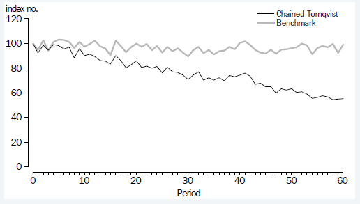
- Indirect (chained) bilateral price indexes compare prices and quantities from consecutive time periods (e.g. period 0 to 1, period 1 to 2) which can be chained together to form a continuous series. While indirect bilateral methods address the item attrition issue observed with direct comparisons, they suffer from a 'chain drift' problem where the index fails to return to parity after prices and quantities revert back to their original values. 'Chain drift' is caused by quantities spiking when consumers stock up goods that are on sale, and not returning to their normal level immediately after the sales period (Ivancic, Fox and Diewert 2011; van der Grient and de Haan 2011). An example of downward ‘chain drift’ is provided in Figure 15.1 for laundry cleaning products which shows the chained Törnqvist falling over 40 percent, while the benchmark price series reports no price change.
Figure 15.1 The 'chain drift' problem
15.7 The limitations of traditional bilateral index formulae have motivated research by NSOs and academics into new methods for compiling price indexes from transactions data. Typically, multilateral index methods have been used in the spatial context to compare price levels across different geographic regions, however academics and NSOs are proposing they be used to make price comparisons across multiple (three or more) time periods. Multilateral methods have a number of advantages for temporal aggregation including:
- Using a census of products available in datasets;
- Weighting products at the product and elementary level by expenditure share;
- Price indexes that are free of 'chain drift'; and
- Reduced resources to produce indexes.
Methods for compiling transactions data
Background
15.8 Multilateral methods possess a number of desirable qualities, both theoretical and practical, to produce temporal price indexes from transactions data. The following details the practical and methodological decisions for aggregating transactions data in four sub-sections: aggregation structure, multilateral method, extension method and multilateral window length. This discussion returns to the framework established in the Information paper: Making Greater Use of Transactions Data to compile the Consumer Price Index (cat. no. 6401.0.60.003) which linked the ABS Data Quality Framework (DQF) to six main criteria for an NSO to evaluate different multilateral methods (Table 15.1).
| Consideration | Quality dimensions |
|---|---|
| Resources: does this method help facilitate more effective use of human and information resources? | Institutional Environment, Timeliness |
| Theoretical properties: what conceptual properties does the index method have, and how well do these align with the CPI purpose? | Accuracy |
| Transitivity: to what extent is the index transitive? | Accuracy, Coherence |
| Characteristicity: to what extent are price comparisons relevant to the time periods being compared? | Accuracy, Relevance |
| Flexibility: what scope is there to use or adapt the method for new statistical products or data sources? | Coherence, Institutional Environment |
| Interpretability: how easy is it to understand the method and the price movements it calculates? | Interpretability |
Product definition
15.9 The definition of a homogeneous product where the calculation of a unit value occurs remains largely consistent with previous practices in the CPI. The ABS defines products using product classifications provided by Australian proprietors known as the stock keeping unit (SKU). The unit value is calculated using expenditure and quantity information across all stores from the same proprietor for each capital city in Australia (e.g. SKU ‘xxx’ from Company 1 for Sydney).
15.10 The unit value is calculated on a quarterly frequency to align with the publication frequency of the Australian CPI. The quarterly unit value is calculated using approximately 2.5 months of revenue and quantity data in order to meet the timeliness constraints for publication - this is consistent with current ABS and international practices. This calculation of quarterly unit values differs slightly with previous CPI practice, where unit values were derived at both monthly and quarterly frequencies. Research has shown that the unit value calculation should align with the publication frequency of the CPI (Diewert, Fox and de Haan 2015).
15.11 The calculation of the unit value should occur across products that are considered equivalent from the perspective of a consumer. Research by other NSOs has shown that matched model multilateral indexes can have a downward bias if price increases are missed when the same item is ‘relaunched’ using a different product identifier (Chessa 2016). The issue of relaunches is a known problem when identifying products using barcodes for certain commodities, while the choice of a broader product definition such as SKU (which is an aggregation of multiple barcodes) should mitigate this problem. The ABS will continue to monitor the suitability of defining products using the SKU.
Elementary aggregation
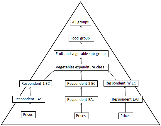
15.12 In order to maximise the use of transactions data using multilateral methods, the ABS has modified the aggregation structure below the published (EC) level. Figure 15.2 details the aggregation structure implemented in the CPI, which uses respondent classes as elementary aggregates (EAs) when these are available from transactions datasets. The direct Törnqvist index formula is used to aggregate respondent EAs together to compile ‘Respondent x EC’ price indexes in order to capture changes in consumer expenditure patterns overtime. ‘Respondent x EC’ indexes are weighted by expenditure (market) share using the Lowe Index formula, with weights being reviewed on an annual basis using both transactions and other data sources.
Figure 15.2 Aggregation structure for transactions data ECs
Image
Description
This diagram includes a pyramid outlining the aggregation structure for transactions data expenditure classes.
This begins at the base of the pyramid with prices. There are three streams which prices is at the base of. Each of the three streams flows up from prices to respondent elementary aggregates.
The first stream flows up from respondent elementary aggregates to respondent 1 expenditure class. The middle stream flows up from respondent elementary aggregates to respondent 2 expenditure class. The final stream flows up from respondent elementary aggregates to respondent ‘n’ expenditure class.
All three streams flow up from respondent 1, 2, and ‘n’ expenditure classes into vegetables expenditure class. This flows up to fruit and vegetable sub-group, which flows up to food group, and finally to all groups. All groups is the top of the pyramid.
15.13 The index structure described in Figure 15.2 includes contributions from transactions data respondents only. The 28 ECs that have this index structure are provided below in Table 15.2. The motivation to compile these ECs using transactions data only is based on evidence of high expenditure (market) share, as well as the resources required to maintain a high quality non-transactions data index component.
| EC |
|---|
| Beef and veal |
| Bread |
| Breakfast cereals |
| Cakes and biscuits |
| Cheese |
| Cleaning and maintenance products |
| Coffee, tea and cocoa |
| Eggs |
| Fish and other seafood |
| Food additives and condiments |
| Fruit |
| Ice cream and other dairy products |
| Jams, honey and spreads |
| Lamb and goat |
| Milk |
| Oils and fats |
| Other cereal products |
| Other food products n.e.c. |
| Other meats |
| Other non-durable household products |
| Personal care products |
| Pets and related products |
| Pork |
| Poultry |
| Snacks and confectionery |
| Tobacco |
| Vegetables |
| Water, soft drinks and juices |
Multilateral method
15.14 In recent years there has been an increase in the range of multilateral methods proposed for use in CPI aggregation when using transactions data. The Information paper: Making Greater Use of Transactions Data to compile the Consumer Price Index (cat. no. 6401.0.60.003) outlines research by the ABS into four multilateral methods considered for implementation into the Australian CPI(footnote 1) . These methods were:
- Weighted Time Product Dummy (TPD)
- Geary-Khamis (GK)
- Quality adjusted unit value using TPD (QAUV_TPD)
- Gini, Eltetö, Köves and Szulc (GEKS)-Törnqvist²
15.15 Testing the different multilateral methods in practice, the ABS found little difference in the empirical results generated from each different multilateral method. Comparing the different methods to the framework described in Table 15.1, the ABS preferred method for compiling price indexes using transactions data is the GEKS-Törnqvist. The two main criteria that differentiate the GEKS-Törnqvist from the other multilateral methods are its theoretical properties (economic approach to index numbers) and interpretability (based on bilateral index number theory). To remedy the sensitivity of the GEKS-Törnqvist to products with atypical prices and small quantities (clearance prices), the ABS uses filters to remove these products from index compilation. The exclusion of products at clearance prices is consistent with current practices adopted in the CPI.
15.16 The GEKS-Törnqvist method takes the geometric mean of the ratios of all bilateral Törnqvist indexes (calculated using the same index number formula) between a number of entities. For spatial indexes these entities are generally countries, while for price comparisons across time, the entities are time periods.
15.17 The bilateral index formula chosen for the Australian CPI is the Törnqvist index which can be expressed as:
\(P^{0,t}_{T}=\prod ^n_\limits {i=0}\Bigg[\frac{p^t_i}{p^0_i}\Bigg]^{\frac{s^t_i+s^0_i}{2}} \space \space \space \space \space (15.1)\)
where,
\(P^{0,t}_{T} = \) Törnqvist index between periods \(0\) and \(t\)
\(p^t_i =\) price of item \(i\) in period \(t\)
\(p^0_i=\) price of item \(i\) in period \(0\)
\({\frac{s^t_i+s^0_i}{2}}=\) average expenditure share of item \(i\) across periods \(0\) and \(t\)
15.18 The GEKS-Törnqvist is calculated as the geometric mean of the ratios of all matched-model Törnqvist bilateral indexes ( \(p^{l,0}\) and \(p^{l,t}\)) where each period is taken in turn as the base (de Haan 2015). The GEKS-Törnqvist method can be expressed as:
\(p_{GEKS}^{0,t}=\prod^T_\limits {l=0}\big[\frac{p^{l,t}}{p^{l,0}} \big] ^{\frac{1}{T+1}} \space \space \space \space \space (15.2)\)
\(P^{0,t}_{GEKS}=\) \(GEKS\) index between periods \(0\) and \(t\)
\(p^{l,0}=\) Törnqvist index between periods \(l\) and \(0\)
\(p^{l,t}=\) Törnqvist index between periods \(l\) and \(t\)
15.19 An example of calculating the GEKS-Törnqvist index across a three period multilateral window is provided below in Figure 15.3. Each row in the figure (or ratio term in the brackets) uses a Törnqvist index to measure price change between periods \(0\) and \(1\), where the base period changes for each row (ratio) whilst the comparison period remains constant. The GEKS then takes the geometric average of these three measures of price change between periods \(0\) and \(1\).
Figure 15.3: Example of GEKS-Tornqvist index
Image
Description
This image show the GEKS-Törnqvist index across a three period multilateral window. Each row in the figure (or ratio term in the brackets) uses a Törnqvist index to measure price change between periods 0 and 1, where the base period changes for each row (ratio) whilst the comparison period remains constant. The GEKS then takes the geometric average of these three measures of price change between periods 0 and 1.
Extension method
15.20 When multilateral methods are used to produce a temporal index, each bilateral price comparison depends on prices observed in other periods of the multilateral comparison window. As a result, incorporating a new period into the multilateral comparison window may revise previous price indexes, which is unacceptable for CPI purposes. To resolve this, researchers and NSOs have developed methods for using the latest multilateral index incorporating the latest data to update the published index series.
15.21 The ABS has considered a range of methods for extending the time series. These can be characterised into the following two groups³:
- The direct (annual) extension: method proposed by Chessa (2016). This involves extending the multilateral estimation window from some (annually) fixed base period as each new period becomes available, and using the price change between the base period and the new period to extend the series
- Rolling window methods inspired by Ivancic, Diewert and Fox (2011), which all involve calculating a new multilateral index using a window of fixed length as each new period becomes available. Having chosen some splice period common to the current and previous windows, the series is extended using the ratio of the price change between the splice period and the current period (using the current window) and the price change between the splice period and the previous period (using the previous window). Choosing the splice period to be the previous period yields a movement splice (Ivancic, Diewert and Fox 2011); choosing the start of the current window yields a window splice (Krsinich 2016); choosing the midpoint of the current window yields a half splice (de Haan 2015). Algebraically, the published index movement from the previous period (t -1) to the current period (t) can be expressed as:
\(p^{t-1,t}=\frac{p^{s,t}_M(current)}{p^{s,t-1}_M(previous)}\space \space \space \space \space (15.3)\)
where:
\(p^{s,t}_M(current)=\) price movement between the splice period \(s\) and \(t\) based on the current multilateral
\(p^{s,t-1}_M(previous)=\) price movement between \(s\) and \(t-1\) based on the previous multilateral window
15.22 While each of the rolling window methods above uses one specific splice period, Diewert and Fox (2017) have endorsed a mean splice rolling window method - initially proposed by Ivancic, Diewert and Fox (2011) - which involves extending the index using the geometric mean of the indexes produced from all possible choices of splice period. Using the notation above, the mean splice extension can be expressed algebraically as:
\(p^{t-1,t}=\prod ^{t-1}_ \limits {s=t-T}\Bigg(\frac{p^{s,t}_M(current)}{p^{s,t-1}_M(previous)}\Bigg)^\frac{1}{T} \space \space \space \space \space (15.4)\)
where the multilateral window length is \(T+1\) periods, so the current and previous periods overlap between \(t-T\) and \(t-1\).
15.23 The ABS has chosen the mean splice motivated by the following factors:
- Conceptually, it seems more natural to make the results independent of the choice of splice period by using all the periods they have in common, rather than choosing a single splice period.
- Empirically, the mean splice appears more robust - while the half splice mitigates systematic quality adjustment bias, choosing an alternative splice period close to the midpoint can give quite different results.
15.24 An example of the mean splice is provided below for a rolling window (length of five periods), where the price movement between periods four and five is estimated by taking the geometric mean of all ratios of GEKS indexes where each common splice period between window one and window two is taken in turn as the base (i.e. one, two, three and four). It can be shown that the mean splice effectively makes a small implicit revision to price movements early in the current window and a large implicit revision to price movements later in the current window. This mitigates the effect of both new and disappearing products, similar to the half splice.
Figure 15.4: Mean splice across rolling multilateral window
Image
Description
This image provides and example of the mean splice for a rolling window (length of five periods), where the price movement between periods four and five is estimated by taking the geometric mean of all ratios of GEKS indexes where each common splice period between window one and window two is taken in turn as the base (i.e. one, two, three and four). It shows that the mean splice effectively makes a small implicit revision to price movements early in the current window and a large implicit revision to price movements later in the current window. This mitigates the effect of both new and disappearing products, similar to the half splice.
Multilateral window length
15.25 The decision to implement a multilateral method requires an NSO to specify the number of time periods used for price comparisons. Most research involving rolling window approaches has recommended a minimum of one year and one period (i.e. five quarters, 13 months) to account for products seasonal availability, though there is currently no consensus on the optimal length of the multilateral window.
15.26 The choice of multilateral window length is a trade-off between two criteria - characteristicity and transitivity. If the multilateral window is too long, then the index could suffer from a loss of characteristicity where price change in the past may disproportionally impact recent inflation estimates. If the multilateral window is too short, the index may suffer from the ‘chain drift’ problem. Empirical testing of different window sizes is necessary to assist with this decision.
15.27 The Information paper: Making Greater Use of Transactions Data to compile the Consumer Price Index (cat. no. 6401.0.60.003) presented results that used a window size of two years and one period (i.e. nine quarters) as the preferred window length - this was based on empirically testing various estimation windows compared to each other (as well as their proximity to different ‘full’ reference price series). Empirical testing by the ABS showed that varying the length of the estimation window generally made little difference to the price series generated. The multilateral window length is two years and one period.
Consultation and future direction
15.28 The ABS undertook broad consultation regarding the implementation of multilateral methods to compile the Australian CPI. This commenced with the release of the Information paper: Making Greater Use of Transactions Data to compile the Consumer Price Index (cat. no. 6401.0.60.003), published 29 November 2016. Following this paper, the ABS sought user and stakeholder input to resolve the outstanding methodological challenges.
15.29 The ABS has collaborated with international experts and NSOs to resolve outstanding methodological issues. Additionally, the ABS conducted bilateral and multilateral consultations with key stakeholders, including: the Reserve Bank of Australia; the Treasury; Department of Social Services; Department of Finance; Department of Prime Minister and Cabinet; and State Treasuries. In all instances, experts, NSOs and stakeholders were supportive of maximising the use of transactions data to compile the CPI using multilateral methods.
15.30 The ABS will continue to monitor methodological developments in the use of transactions data to compile price indexes, as well as continue to conduct research into remaining practical issues including text mining, hedonics indexes, automated text mapping and the use of multilateral methods for aggregating prices ‘web scraped’ from online.
References
Australian Bureau of Statistics (ABS) 2016. Making Greater use of Transactions Data to Compile the Consumer Price Index. cat. no. 6401.0.60.003. ABS, Canberra.
Chessa, A. G. 2016. A new methodology for processing scanner data in the Dutch CPI. Eurostat review of National Accounts and Macroecnomic Indicators, 1, 49-70.
Diewert, E. W. 1995. Axiomatic and Economic Approaches to Elementary Price Indexes. Discussion Paper No. 95-01; Department of Economics, University of British Columbia.
Diewert, E. W., Fox, K. J. & de Haan, J. 2016. A newly identified source of potential CPI bias: Weekly versus monthly unit value price indexes. Economics Letters, 141, 169-172.
Diewert, E.W. & Fox, K.J. 2017. Substitution Bias in Multilateral Methods for CPI Construction using Scanner Data. Discussion Paper No. 17-02; Vancouver School of Economics, University of British Columbia.
de Haan, J. 2015. A Framework for Large Scale Use of Scanner Data in the Dutch CPI. Paper presented at the fourteenth Ottawa Group meeting. Tokyo, Japan.
de Haan, J. and van der Grient, H. 2011, Eliminating Chain Drift in Price Indexes Based on Scanner Data, Journal of Econometrics 161, 36-46.
International Labour Organization (ILO) 2004. Consumer Price Index Manual: Theory and practice, International Labour Office, Geneva.
Ivancic, L., Fox, K. J. & Diewert, E. W. 2011. Scanner data, time aggregation and the construction of price indexes. Journal of Econometrics, 161, 24-35.