| Item | Comment |
|---|---|
| Output | |
Output is the production of goods and services for use as inputs into the production process of an industry, or as final demand. Own production and use of some energy products and transportation not separately invoiced are not shown separately and are included as part of an industry’s output. The main data sources used to compile output in the Supply and Use tables are the Economic Activity Survey, Government Finance Statistics (GFS) and the Australian Prudential Regulatory Authority (APRA). Industry-specific data sources may also be used. Chapter 9 outlines, in detail, the data sources and methods used to compile output by industry. A number of adjustments are made to the source EAS data in the S-U tables, namely:
| |
| Intermediate consumption | |
Intermediate consumption consists of the value of goods and services consumed as inputs to the production process. The main data sources used to compile intermediate consumption in the Supply and Use tables are the Economic Activity Survey and Government Finance Statistics. A number of adjustments are made to the source EAS data in the S-U tables, namely:
| |
| Household final consumption expenditure | |
Household final consumption expenditure (HFCE) consists of the expenditure incurred by households on individual consumption goods and services. The HFCE benchmark data is sourced from the periodic Retail and Wholesale Industry Surveys (RIS/WIS) and the Household Expenditure Survey (HES). The annual estimate is the sum of the four quarters for years when the RISWIS and HES data are not available. Between survey years, the Retail Trade survey is used as an indicator for merchandise items, and a range of relevant indicators are used for services (see Chapter 10 on GDP(E) for more detail). | |
| Government final consumption expenditure | |
Government final consumption expenditure (GFCE) consists of the expenditure incurred by general government on both individual consumption goods and services and collective consumption services. The main data source used to compile GFCE in the Supply and Use tables is the Government Finance Statistics. GFS data are classified according to the General Purpose Classification (GPC) and the Local Government Purpose Classification (LGPC). | |
| Gross fixed capital formation | |
Gross fixed capital formation (GFCF) is equal to the total value of a producer’s acquisitions, less disposals, of fixed assets plus capital work done on own account plus certain additions to the value of non-produced assets realised by the productive activity of institutional units (i.e. land improvements). Estimates of GFCF are primarily disaggregated between the private and public sectors. There are a range of data sources used to compile private GFCF in the Supply and Use tables, including:
The main data source used to compile public GFCF in the Supply and Use tables is the Government Finance Statistics. GFCF is classified by type of asset. | |
| Changes in inventories | |
Changes in inventories are defined to include changes in holdings of goods for sale (whether of own production or purchased for resale), work-in-progress and raw materials to be used as intermediate inputs into production. The main data sources used to compile total changes in inventories in the Supply and Use tables are the Economic Activity Survey and Government Finance Statistics. | |
| Exports of goods and services | |
Exports of goods and services are defined as being domestically produced output acquired by non-residents. The primary source used to compile exports of goods is the ABS International Merchandise Trade Statistics. Balance of Payments adjustments to coverage, timing and valuation are applied, using data from the Survey of International Transport Enterprises, the Reserve bank of Australia and the Survey of International Trade in Services. The principal sources used to compile exports of services are the ABS International Merchandise Trade Statistics, the cost, insurance and freight/free on board (c.i.f./f.o.b.) model and the Survey of International Trade in Services (SITS. | |
| Imports of goods and services | |
Imports of goods and services are defined as being the outputs produced by non-residents but acquired by residents. The principal source used to compile imports of goods is the ABS International Trade Statistics. Balance of Payments adjustments to coverage, timing and valuation are applied, using data from the Survey of International Transport Enterprises; Reserve Bank of Australia (RBA); and the Survey of International Trade in Services. The principal sources used to compile imports of services are the ABS International Merchandise Trade Statistics, the cost, insurance and freight/free-on-board (c.i.f./f.o.b.) model and the Survey of International trade in services. | |
| Compensation of employees | |
Compensation of employees is defined as being the total remuneration, in cash or in kind, payable to an employee in return for work done. It comprises wages and salaries and employers' social contributions. The main data sources used to compile compensation of employees in the Supply and Use tables are the Economic Activity Survey; Survey of Employment and Earnings (SEE); Survey of Major Labour Costs; and the Australian Prudential Regulatory Authority. | |
| Gross operating surplus/gross mixed income | |
Gross operating surplus (GOS) is defined as being the income from production of corporate enterprises, while gross mixed income (GMI) is the income from production of unincorporated enterprises. GOS is calculated as gross value added less compensation of employees less net taxes on production and imports for all industries/institutional sectors except:
GMI is derived as the residual once all of the other institutional sectors GOS is estimated (i.e. private non-financial corporations, public non-financial corporations, general government and financial corporations GOS). | |
| Taxes less subsidies on production and imports | |
Taxes on production and imports consist of taxes on products (i.e. taxes on goods and services when they are produced, delivered or sold and duties on imports) and other taxes on production (i.e. taxes related to the payroll, land taxes, taxes on pollution, stamp duties (not including those on real estate or road vehicles), etc.). Subsidies on production consist of subsides on products (i.e. subsidies on goods and services when they are produced, delivered or sold) and other subsidies on production (i.e. subsidies related to the payroll or workforce). The main data source used to compile taxes less subsidies on production and imports in the Supply and Use tables is the Government Finance Statistics. | |
Chapter 22 Input-Output Tables
Introduction
22.1 The input-output tables form an integral part of the ASNA. They present a comprehensive picture of the supply and use of all products in the economy, and the incomes generated from production. They also provide a much more detailed disaggregation of gross domestic product than is available in the national income, expenditure and production (GDP) accounts. This chapter provides a detailed description of the I-O tables, their importance within the overall ASNA, the compilation process, and how they relate to the rest of the accounts. Two kinds of I-O tables are referred to in national accounting and economic analysis:
- supply-use tables (see Chapter 7 for a full description of how S-U tables are used to benchmark the ASNA); and
- input-output tables, including symmetric I-O tables (product by product or industry by industry matrices which combine supply and use into the one table, with identical classifications of products or industries applied to both rows and columns).
22.2 The integration of 'input-output' in the overall system of national accounts is an important feature of the ASNA. Its role in the ASNA is primarily related to the goods and services accounts and to the shortened sequence of accounts for industries. The I-O tables serve to provide a more detailed basis for analysing industries and products through a breakdown of the production account, leading to the symmetric input-output table. 'Symmetric' means that the same classifications or units (e.g. the same groups of products) are used in both rows and columns. When the number of rows of products and columns of industries happens to be equal, they are referred to as square (not symmetric) I-O tables. However, I-O tables are most often rectangular (having more products than industries).
22.3 The I-O and S-U tables serve two purposes: statistical and analytical. They provide a framework for checking the consistency of statistics on flows of goods and services obtained from quite different kinds of statistical sources - industrial surveys, household expenditure surveys, investment surveys, foreign trade statistics, etc. The ASNA, and the I-O tables in particular, serves as a coordinating framework for economic statistics, both conceptually for ensuring the consistency of the definitions and classifications used and as an accounting framework for ensuring the numerical consistency of data drawn from different sources. The I-O framework is also appropriate for data estimation purposes, and for detecting weaknesses in data quality and estimation. By providing information on the structure of, and the nature of product flows through the economy, the I-O tables assist in the decomposition of transactions into prices and volumes for the calculation of an integrated set of price and volume measures. As an analytical tool, input-output data are conveniently integrated into macroeconomic models in order to analyse the link between final demand and industrial output levels. Input-output analysis also serves a number of other analytical purposes or uses, which are discussed further in the sections below.
22.4 I-O tables are not revised once they have been finalised. They are not compiled as a time series but rather are a point in time reflection of the economy. The rest of the national accounts (e.g. the S-U tables and the GDP accounts) may be revised for all periods whenever an historical revision is undertaken, and therefore are a consistent time series. Therefore, an I-O table can only be considered current with the published national accounts within a year of their publication.
22.5 Various tables are included under the broad heading of I-O tables. Each of these tables provides detail that underlies the aggregates recorded in the gross domestic product account. These summary accounts are focused on the end result of economic activity, whereas the I-O tables provide detailed dissections of that activity, industry to industry flows and by showing intermediate transactions they enhance the description of productive activity within the economy.
The structure of the I-O tables
22.6 The I-O tables are sourced from the S-U tables, and the concepts and definitions used are the same as elsewhere in the ASNA. Issues of particular importance to the I-O tables include statistical units and the distinction between primary and secondary activities.
22.7 The ABS uses an economic statistics model to describe the characteristics of units, and the structural relationships between businesses. Businesses with a simple structure are classified by their Australian Business Number (ABN) on the Australian Business Register (ABR), maintained by the Australian Taxation Office. Businesses with a more complex structure (i.e. where the ABN is not suitable for ABS statistical requirements) are maintained on the ABS Maintained Population register (ABSMP), through direct contact with the business. These units comprise the Enterprise Group, the Enterprise and the Type of Activity Unit (TAU). The TAU represents a grouping of one or more business entities for which a basic set of financial production or employment data can be reported.
22.8 When a unit engages in more than one type of production, the primary production is the activity for which gross value added is the greatest for that unit. The production reported by a unit may include both primary and secondary production. The output of an industry may be a number of products that are jointly produced (e.g. natural gas linked to crude oil). In this case primary products may be distinguished by the principal product with the smaller output treated as secondary production.
22.9 I-O tables can be compiled for industries or products but they are both similar in theory. The distinguishing characteristics of analytical I-O tables are that they are square and symmetric, and they differ from the S-U tables in that the transactions are valued at basic prices rather than purchasers’ prices. The I-O tables provide detailed information about the supply and use of products in the Australian economy and about the structure and inter-relationship between Australian industries.
22.10 Table 22.1 provides a summary of the different dimensions and values shown in the published I-O tables. Detailed information on the content of each published table is provided below the summary table.
| Table No. | Type of table | Row | Column | Value | |
|---|---|---|---|---|---|
| 1 - 4 | Basic tables | Product | Industry | Current Price | |
| 5 | Derived table | Industry | Industry | Current Price | |
| 6 - 7 | Derived tables | Industry | Industry | Coefficient | |
| 8 | Derived table | Industry | Industry | Current Price | |
| 9 - 10 | Derived tables | Industry | Industry | Coefficient | |
| 17 | Derived table | Industry | Primary Input | Percentage | |
| 19 | Derived table | Industry | Ratios | Coefficient | |
| 20 | Derived table | Industry | Employment | No. of persons | |
| 21 | Basic table | Product | Margin/Non-margin | Current Price | |
| 23 -39 | Basic tables | Product | Industry | Current Price | |
| 40 | Correspondence tables | ||||
Basic tables of I-O
22.11 The basic tables of I-O are aggregations of the various components of GDP. The most significant feature of these tables is that they are not symmetrical in that the dimension of the columns differs from dimension of the rows.
22.12 There are four main basic tables used to compile the I-O tables:
- Supply table – shows the output of domestic industries and imports classified across columns, and products classified across rows. The largest values are found on the leading diagonal as industries specialise in their primary products. The columns in the supply table show the products each industry produces, and the extent to which industry specialises in the production of its primary products, as well as the product composition of imports.
- Use table – shows the product groups and primary inputs in the rows, and industries and final use categories in the columns. The rows show the total supply of products, whether locally produced or imported, and show how these products are used by industries as intermediate inputs to production or consumed as final demand by category. At the bottom of the table, the rows show the primary inputs purchased by industries, and by final demand. Reading down the columns shows that you can read the inputs (intermediate and primary) into each industry, and the composition of each final demand category. Therefore, all flows of goods and services in the economy are covered.
- Imports table – shows in the columns the industries to which imported products would have been primary if they had been produced in Australia, and in rows the usage of these products by industry and final demand category. This breakdown is only shown for competing imports, or those products which are produced domestically and imported, so that substitution between domestically produced products and imports is possible. The disposition is not shown for complementary imports, which by definition are products that are not domestically produced. Since the 2001-02 I-O tables, ABS has not measured complementary imports, and assigns all imports as competing.
- Margins table – shows the difference between the basic price and the purchaser’s price of all flows in the use table. Table 4 shows the decomposition of flows at purchaser prices into basic prices, net taxes on products and the sum of all trade and transport margins. Tables 23 to 39 show the detailed disposition of each type of margin, product taxes by type, and product subsidies, to intermediate use and final use categories.
22.13 These four main basic tables make up a record of the estimated flows which occur in the production process. However, the use table is not symmetric which makes it unsuitable for some forms of analysis. This problem is solved by converting the use table to an industry-by-industry flow table by adjusting the rows to show industry use of industry output, rather than products. The ABS does not produce product-by-product flow tables.
22.14 Table 22.2 provides a summary of the basic I-O tables published by the ABS.
| Table No. | Description | |
|---|---|---|
| 1 | Australian production by product group by industry
| |
| 2 | Input by industry and final use category and Australian production and imports by product group
| |
| 3 | Imports - supply by product group and inputs by industry and final use category
| |
| 4 | Reconciliation of flows at basic prices and at purchasers' prices by product group
| |
| 21 | Composition of supply of products containing margins
| |
| 23 | Wholesale margin on supply by product group by using industry and final use category
| |
| 24 | Retail margin on supply by product group by using industry and final use category
| |
| 25 | Restaurants, hotels and clubs margin on supply by product group by using industry and final use category
| |
| 26 | Road transport margin on supply by product group by using industry and final use category
| |
| 27 | Rail transport margin on supply by product group by using industry and final use category
| |
| 28 | Pipeline transport margin on supply by product group by using industry and final use category
| |
| 29 | Water transport margin on supply by product group by using industry and final use category
| |
| 30 | Air transport margin on supply by product group by using industry and final use category
| |
| 31 | Port handling margin on supply by product group by using industry and final use category
| |
| 32 | Marine insurance margin on supply by product group by using industry and final use category
| |
| 33 | Gas margin on supply by product group by using industry and final use category
| |
| 34 | Electricity margin on supply by product group by using industry and final use category
| |
| 35 | Net taxes on products by product group by using industry and final use category
| |
| 36 | Goods and services tax on products by product group by using industry and final use category
| |
| 37 | Duty on products by product group by using industry and final use category
| |
| 38 | Taxes on products nei by product group by using industry and final use category
| |
| 39 | Subsidies on products by product group by using industry and final use category
| |
Derived tables of I-O
Changes made to Table 22.2 Basic tables published by the ABS
From 28/10/2024,
The title of Table 1 has been changed to reflect the latest issue of Australian National Accounts: Input-Output Tables.
22.15 Derived tables differ from the basic tables in I-O in that they are symmetric so that the dimensions of the columns and rows are the same. The dimension is either product by product or industry by industry. In Australia the derived I-O tables are industry by industry.
22.16 Another feature of the derived table is that they are not simply aggregations of the components. Some further calculations are applied in order to produce the tables namely the derivation of coefficients.
22.17 Table 22.3 depicts the industry-by-industry table. A row in the table shows the disposition of the output of an industry group and a column shows the origin of inputs into an industry and final use category. The output of an industry equals the sum of its inputs including its primary inputs so the column total must equal the row total.
Table 22.3 Industry by industry flow matrix
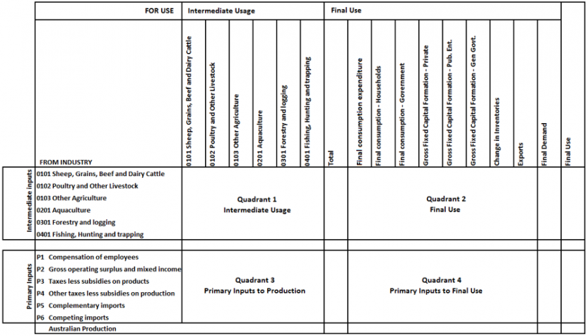
22.18 Table 22.3 shows the basic structure of an industry-by-industry table with direct allocation of imports (as is published in Table 5 of the I-O tables) where imports are allocated to the using industries. The flows between the domestic industries are:
- Quadrant 1 – this is referred to as the inter-industry quadrant where each column shows the intermediate inputs into an industry in the form of products produced by other industries and itself. Each row shows how the output of an industry has been used by itself and other industries as part of their production process;
- Quadrant 2 – shows the disposition of output to final use categories by industry group;
- Quadrant 3 – shows the primary inputs to production (compensation of employees, gross operating surplus and gross mixed income, imports and net taxes on production); and
- Quadrant 4 – shows the disposition of primary inputs to final demand categories.
22.19 The sum of quadrants 1 and 2 shows the total usage of goods and services produced by each industry. Total usage equals total supply, with final demand including change in inventories, which may be positive or negative.
22.20 The sum of quadrants 1 and 3 shows the total inputs required to produce the outputs of each industry group. Total inputs equals total supply or outputs, with primary inputs including gross operating surplus and gross mixed income, which can conceptually be positive or negative.
22.21 Table 8 of the I-O tables is an industry-by-industry flow table with indirect allocation of imports. This table shows:
- supply by industry group, including Australian production and products which are imported; and
- the inputs into an industry’s production, reflecting the technological relationships between all inputs into the industry, whether domestically produced or imported.
22.22 In order to balance the table, the row for competing imports is shown below the Australian production; that is, showing total supply (row total) for each industry as being equal to the corresponding total uses (column total). For each column, this row shows the value of imports competing with the output of each industry. This presentation results in the double entry for imports in the table to reconcile total supply and total uses. In a table with direct allocation of imports, the competing imports row is shown above the Australian production row, and shows, for each industry, the total intermediate use of imports by the industry.
22.23 The difference between the direct and indirect allocation of imports is discussed in the allocation of imports section (paras.22.55-22.61).
22.24 The following table provides a summary of the derived I-O tables published by the ABS:
| Table No. | Description |
|---|---|
| 5 | Industry by industry flow table (direct allocation of imports)
|
| 6 | Direct requirement coefficients (direct allocation of imports)
|
| 7 | Total requirement coefficients (direct allocation of imports)
|
| 8 | Industry by industry flow table (indirect allocation of imports)
|
| 9 | Direct requirement coefficients (indirect allocation of imports)
|
| 10 | Total requirement coefficients (indirect allocation of imports)
|
Additional published tables
There are four additional tables that are published which are not basic or derived I-O tables. The following table provides a summary of them:
| Table No. | Description |
|---|---|
| 17 | Primary input content (total requirements) per $100 of final use by industry
|
| 19 | Specialisation and coverage ratios by industry
|
| 20 | Employment by industry
|
| 40 | Industry and product concordances
|
Homogeneity assumption
22.26 In Quadrant 1, a row or column is said to refer to an industry; however, a row or column can refer to a product (or group of products) rather than an industry. The structure of products or industries is important in the use of the I-O tables. It is desirable that each product or industry changes as little as possible over time, and that each industry produces a single output, with a single input structure. This approach implies that all products produced by an industry are perfect substitutes for each other or are produced in fixed proportions. It also implies that the input structure does not vary in response to changes in the product mix, and that there is no substitution between the products of different groups of products or industries. This is known as the homogeneity assumption; however, it is not fully supported in the ABS I-O tables.
22.27 The stability of coefficients is affected by the interaction of two factors: (a) the aggregation of products with different input structures; and (b) changes in the product group mix over time. This becomes important when the data sources for the I-O coefficients are infrequent, such that it is necessary to assume that observed coefficients apply in the following years, at least as a starting point. This problem arises in industries producing a range of products that have different input structures.
22.28 There is significant aggregation even in large I-O tables, leading to a departure from these objectives, and affecting the homogeneity of products or industries. There are two ways the aggregation can be made: (a) grouping by industries to create an industry-by-industry table (the ABS approach); or (b) grouping by products to create a product-by-product table. The two methods result in differing impacts on homogeneity, with different implications for the analytical use of the tables. There is no complete solution for the aggregation problem, but appropriate grouping can keep errors to acceptable limits. The groups used are partly dependent on industry classifications, and the practical process of compiling the I-O tables.
22.29 At first sight, the solution to the grouping problem is to narrowly define product groupings. However, this could result in the tables becoming too complicated for users, and would take too long to compile, particularly as the ABS is now producing I-O tables every year. Even with narrower product groupings, there would be instances where a TAU produced products classified to different groups of products, and it would not be practical to split details to different groups. Confidentiality would also become a problem in some industries, as the products covered in a group became more specific.
22.30 For industries, the homogeneity assumption will not be fully met as some industry groups produce a wide range of products at the industry-group level. Similar to above, the classification of industries as establishments or TAUs would make the tables too complicated; the tables would take too long to compile; and there would be confidentiality issues. Grouping industries will still result in secondary production, where the products have different input structures. For example, if the basic iron and steel industry also produces non-ferrous castings, the input structure for this column will show the use of non-ferrous metals, and the corresponding row will show sales of products to industries using non-ferrous castings. These results may not be suitable for users interested only in iron and steel products. The requirements calculated from this table could be misleading, unless the production of secondary products forms a fixed proportion of the industry's output. The proportion of product mix should remain constant where secondary products are jointly produced, or the secondary product is a by-product of the primary production; there is often no correlation between primary and secondary products.
22.31 The extent of secondary production by an industry depends on the range of products produced by individual establishments, and whether the industries are grouped into large numbers of narrowly defined industries, or a small number of broadly defined industries. Where industries are narrowly defined, a large proportion of the products will be produced by industries to which the products are not primary. This conflicts with both the homogeneity requirement and the non-substitution requirement. Where significant proportions of a product can be substituted by products produced by a different industry, there is a weak link between the demand for a product and the output of a single industry. Combining some of these industries could improve homogeneity in one respect, at the expense of creating a more heterogeneous product mix.
Grouping of products and industries
22.32 The availability of source data will ultimately affect the grouping of products or industries. Detailed information of sales or output of products is normally available, but information on costs may not be available. In some cases, only input structure detail may be available. A rolling program of case studies is used to gather detailed data on companies’ input and output structures, by direct interview with companies, in order to assist with this problem. In the past, economic activity by some industries was redefined to more appropriate industries to limit the impact of secondary production on the tables, but this is no longer done in order to reflect how production occurs in the economy.
22.33 Regardless of whether products or industries are used in quadrant 1, the same processes are followed to assemble the data. It is necessary to record the product flows in a way that is suitable to compile I-O tables. The same information is required for each product or product group:
- the origin or source of supply, domestic supply by industry, and imports;
- the use of the product, intermediate usage by industry and final demand by category; and
- the difference (margins, taxes and subsidies on products) between the basic price and purchaser's price for each product.
22.34 The supply of imports must be classified in the same way as Australian production. Imports data is sourced from Customs data. These data are initially classified according to the Harmonised Tariff Item Statistical Code (HTISC) which is then concorded to the Input-Output Product Classification. The data enters the I-O tables as a vector and is allocated to the industry to which the imported product is primary.
Deviations from International Standards
22.35 The I-O tables are an analytical tool which is compiled using the balanced S-U tables as a starting point. They can deviate to an extent from ASNA and 2008 SNA treatments in order to serve particular analytical purposes. The two main deviations are described below in more detail. They are:
- the 1968 SNA transport margin adjustment; and
- the c.i.f./f.o.b. adjustment.
22.36 The following is the list of aggregates where consistency is ensured between the I-O tables and the rest of the national accounts:
- household final consumption expenditure;
- government final consumption expenditure (total only);
- private gross fixed capital formation (total only);
- public corporations gross fixed capital formation (total only);
- general government gross fixed capital formation (total only);
- changes in inventories (total only);
- exports (total only including re-exports);
- imports (total only);
- compensation of employees (total only);
- gross operating surplus and gross mixed income (total only);
- taxes less subsidies on products;
- other taxes less subsidies on production and imports;
- income from dwelling rent - total gross rent;
- income from dwelling rent - consumption of financial services; and
- industry value added (industry level).
The 1968 SNA transport margin adjustment
22.37 The 1968 SNA Transport Margin Adjustment (SNA68 TMA) aims to capture the transport charges for goods delivered by a third party, arranged by the producer without a separate invoice. I-O tables depart from the 2008 SNA in the definition of output at basic prices due to user requirements. SNA68 TMA ensures the same product is not being valued differently depending regardless of whether the producer charged separately for the delivery of the product or not.
22.38 The transport charges are removed from Australian production and added to the transport margins and thus reducing supply at basic prices. The amount of the adjustment is sourced from the Economic Activity Survey (EAS) at the ANZSIC06 class level and aggregated to IOIG and disaggregated to product. The adjustment is applied to the products in four divisions; Agriculture, Forestry and Fishing; Mining; Manufacturing; and Arts and Recreation Services (applied to only one product of artistic originals).
22.39 SNA68 TMA is only applied to primary production of Australian goods; wholly imported goods have zero SNA68 TMA. The adjustment is only applied to five transport margin types; Road, Rail, Water, Air and Stevedoring. For row balancing purposes, the margin allocated to that product is increased respectively as the output is decreased. The increase in the margin columns is offset by a decrease in Australian production at basic price. To balance the margin products in the output matrix, the margin product is increased and the transport non-margin product is decreased to balance the column. To complete the process, the imbalance in the output matrix of the non-margin product is offset with a respective decrease in the Intermediate Use of that product.
22.40 Overall, the supply at basic prices is reduced and the margins increased with the same amount, and supply at purchaser prices remains the same, except for transport non-margin products. There are four quality checks that ensure the adjustment is applied properly:
- no negative supply at BP;
- no negative margins (except in margin products);
- no change in supply at PP except for transport non-margin products; and
- the sum of margins equals zero.
The c.i.f./f.o.b. adjustment
22.41 Each imported good in the input-output tables is valued cost insurance and freight (c.i.f.) since it is the equivalent to the basic price of the same domestic product. However, total imports has to be valued free-on-board (f.o.b.) in accordance with BOP and National Accounts methodology. Transport and insurance services on imported goods may be performed by residents and non-residents. If the latter is a genuine import of services, the former is a domestic output and should not be treated as imports. Two operations are therefore necessary: firstly, to reconcile detailed c.i.f. values with total imports f.o.b., and secondly, to avoid the double counting of resident services:
The c.i.f./f.o.b. adjustment
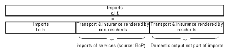
22.42 The total adjustment corresponding to the transport and insurance services rendered by residents is, by construction, negative:
| – transport and insurance services rendered by residents |
| = (imports f.o.b. - imports c.i.f.) + (transport and insurance rendered by non-residents) |
22.43 The UN Handbook of Input-Output Table Compilation and Analysis recommends the presentation of the c.i.f./f.o.b. adjustment as a separate item in the I-O tables. This presentation has not been adopted in the ABS I-O tables, where the adjustment is added to the transport and insurance services rendered by non-residents as explained above. These two items are allocated to non-margin water transport and non-margin air freight products. The sum of these two components is, by construction, negative.
22.44 A negative value in imports is conceptually correct and complies with the UN handbook. Because negative values are incompatible with some analytical models, the ABS also compiles a different view of the tables by re-allocating this negative adjustment on imports to a positive adjustment on exports. The consequence is an increase by the same amount of both imports and exports.
22.45 An alternative view of the I-O tables is also published to support the needs of users who apply the data in large and sophisticated models. The tables mirror the main I-O tables except for the different treatment of the c.i.f./f.o.b. adjustment.
Special treatments adopted in compiling I‑O tables
22.46 The symmetric I-O tables are sourced from the S-U tables, and the concepts and definitions used are the same as elsewhere in the ASNA. Issues of particular importance to the I-O tables include statistical units and the distinction between primary and secondary production.
22.47 The content and meaning of the I-O tables produced depend on some particular aspects of compilation including:
- the treatment of intra-industry transactions; and
- the allocation of imports.
Intra-industry transactions
22.48 Depending on the treatment of intra-industry transactions, the output of an industry can be defined in three different ways according to whether, and to what extent, these transactions are counted as part of the output.
22.49 Firstly, the output of an industry can be defined as the total value of all flows of products produced by the units classified to the industry. All intra-industry flows are included as output when it is defined in this way. Under this definition, for example, the output of the Motor vehicles and parts; Other transport equipment industry consists not only of fully assembled vehicles but also of motor bodies, engines and other components despatched from (or added to inventories by) any unit recognised as a unit for statistical purposes. This definition of output disregards the fact that many of these components will have been incorporated in finished motor vehicles and will have therefore been counted twice. Output calculated according to this definition could be as much as two or three times the value of finished products of the industry.
22.50 A second definition of the output of an industry confines output to products produced by units within the industry and sold outside the enterprise. This definition also results in some duplication because the components manufactured and sold by one enterprise are all counted separately, although they may have been used in a finished product of another enterprise in the same industry and counted again in the value of this product. Moreover, the components despatched from one unit could be omitted entirely or counted either partly or wholly depending on whether they were used by another unit of the same enterprise or by a different enterprise.
22.51 Thirdly, the output of an industry can be defined as net of all intra-industry transactions; that is, excluding not only the transfers between the unit in industry belonging to the same enterprise, but also all flows between units in industry belonging to different enterprises.
22.52 If the third definition of output is used, the I-O table is said to be net and the main diagonal of an industry-by-industry table is empty. If either the first or second definition of output is used the I-O table is said to be gross and there are entries on the main diagonal.
22.53 For 1974–75 and subsequent years, the ABS I-O tables generally include intra-industry flows and can be described as 'gross', as outlined above. This means that the estimates of output can be directly compared with other information about an industry.
22.54 A further consequence of recording intra-industry transactions is that the level of output is unaffected by the number of industries used (i.e. by different levels of industry aggregation). An important exception is the construction industry, in which output was measured on a net basis prior to the 2001-02 tables.
Allocation of imports
22.55 Information regarding the use of imports in the economy is not generally available because it is impractical to collect data on how imported products are used. For analytical purposes, the ABS models the use of imports in the intermediate and final use categories using a number of assumptions. In an indirect allocation of imports approach, imports are not distinguished from domestically produced products and their use is therefore based on their contribution to the total supply. Specific rules also determine the disposition of imports which, by definition cannot be allocated to domestic exports but must be allocated to re-exports.
22.56 Various ways are available to record imports in the I-O tables. The main ones are:
- direct allocation of imports – involves allocating all imports directly to the industries which use them. In this case, all flows recorded in quadrants 1 and 2 refer only to the use of domestic products, and consequently quadrant 1 does not reflect the technological input structure of the industry;
- indirect allocation of imports – involves first recording all imports as adding to the supply of the industry to which they are primary and then allocating this supply along the corresponding row of the table to using industries. The result is that flows in quadrants 1 and 2 contain imported and domestically produced products without distinction. Quadrant 1 then better reflects the technological input structure of the industry and quadrant 2 better reflects the product composition of final demand; and
- direct allocation of complementary imports and indirect allocation of competing imports – this method involves first distinguishing between complementary and competing imports and then allocating the first group directly and the latter indirectly. Complementary imports are defined as those for which no suitable substitute is produced domestically, but determining what is a suitable substitute is largely a matter of judgement. As complementary imports ceased to be separately distinguished from the 2001-02 tables onwards this method is not available in the published ABS I-O tables.
22.57 Each of these methods has advantages from an analytical point-of-view but each also can lead to conceptual and compilation problems.
22.58 Direct allocation of imports is appropriate for many analytical purposes. However, it would be necessary to adjust the imports table and to recalculate the industry-by-industry tables if substitution between imports and domestic production is known to occur, in order to allow for the probable effects of specified import replacement or substitution. In addition, the application of this method requires identification of the destination of each imported product. Although the proportion of imports in total supply (and therefore in total usage) for each product can be established, it may not be known for individual using industries. Of course, it is possible to proceed if one assumes that each using industry draws on imports and domestic production in the average proportions established for the total supply of each product. In the I-O publication, tables with direct allocation of competing imports have been prepared using this assumption. The assumption was applied to detailed working tables which were subsequently aggregated for publication.
22.59 Indirect allocation of imports is appropriate, in the sense that it will result in stable input-output coefficients, where the inputs to the domestic industry to which each imported product is primary are representative of the inputs required to produce the import domestically. Where this is not so, the method will give misleading results. For instance, if coffee (which could be treated as a complementary import) were distributed with the 'other agriculture' product group, an increase in the demand for coffee would necessitate an increase in the output of the 'other agriculture' industry. This, in turn, would require an increase in the inputs to that industry as specified in the published tables unless a specific adjustment is made to the tables. It is easy to compile tables using the indirect allocation method. The initial problem which has to be overcome is matching each imported product with the domestic industry to which the product is primary or would have been primary if it were produced domestically.
Coverage of transactions
22.60 The input-output tables record only those flows of goods and services that have been domestically produced, imported or drawn from domestic inventories during the reference period. Therefore, some transactions are outside the scope of the I-O tables, and are not recorded in them. The most important exclusions are financial transactions, such as loans, interest and the purchases of securities, which are not products in an SNA sense.
22.61 Other transactions have to be modified before they can be included in the tables. For instance, flows of products are commonly reported as sales and purchases, but the I-O tables should record output and usage. Output will differ from sales, and input (or usage) will differ from purchases, by the amount of inventory change (positive or negative) in both cases. Output is calculated as sales plus changes in inventories of finished goods plus changes in inventories of work-in-progress, and input is calculated as purchases less changes in inventories of materials. Changes in inventories are recorded in a separate final demand column in the row of the industry of origin. Entries in this column refer to changes in inventories of both domestically produced and imported products, regardless of whether they are held by producers, dealers or intermediate users.
22.62 Input-output tables include some elements which are not market transactions, such as the imputed rentals of owner-occupied dwellings and some home-produced food, as output for own-final consumption.
22.63 For analytical purposes, they also include own intermediate use of some energy products such as gas or electricity.
22.64 Estimates for own-account computer software and research and development are also included to estimate output, as output for own final use as fixed capital formation.
Valuation of transactions
22.65 The flows in Input-Output tables can be valued in several ways. The choice depends partly on the intended use of the tables and partly on availability of data (including the assumptions that can reasonably be made where data are lacking). The valuation conventions most commonly used are basic prices, producers' prices and purchasers’ prices. They are defined as follows:
- Basic prices – the amount receivable by the producer from the purchaser for a unit of a good or service produced as output, minus any tax payable, and plus any subsidy receivable, on that unit as a consequence of its production or sale. It excludes any transport charges invoiced separately by the producer, and an adjustment is made to exclude delivery charges that are not separately invoiced, organised by the producer and delivered by a third party.
- Producers’ prices – the amount receivable by the producer from the purchaser for a unit of a good or service produced as output, including any tax that is incorporated within the sales price, and excluding any subsidy that reduces the sales price, on that unit as a consequence of its production or sale. It excludes any transport charges invoiced separately by the producer, and an adjustment would be made to exclude delivery charges that are not separately invoiced, however, producer's price is not used in the Australian I-O tables.
- Purchasers’ prices – the amount paid by the purchaser in order to take delivery of a unit of a good or service at the time and place required by the purchaser. It includes any transport charges paid separately by the purchaser to take delivery at the required time and place. GST paid by producers for which input credits are granted is excluded from purchasers' prices.
22.66 The difference between the cost of a product to the purchaser and the basic price receivable by the producer is composed of taxes less subsidies on products and margins such as transport and storage services, marine insurance, and wholesale and retail margins. Regardless of whether the producer or the purchaser initially pays for the margins, the concept of producer's price excludes the margins and the concept of purchaser's price includes them.
Special valuation issues
Basic margins
22.67 If the transactions are valued at basic prices, the margins are recorded as inputs from the appropriate industry (e.g. transport, wholesale trade) to the intermediate users or final buyers. If transactions are valued at purchasers' prices, the value of the margins is added, along with taxes less subsidies on products, to the basic price of the good to which the margins relate. The input into the intermediate or final use category of the transport or wholesale trade industry is reduced by a corresponding amount.
22.68 Whichever method is used, a complicated estimation process will be necessary before the transactions can be valued in one of these ways. First, input and output statistics from economic statistics collections are not available on the same valuation basis. Most output statistics are on an ex-plant or similar basis, but input statistics are normally available at the price paid by the user. Second, margins apply only to those flows of products which have actually passed through the 'margin' industries. Any products delivered directly from producer to user, without intervention of 'margin' industries, are obviously unaffected by margins.
22.69 The incidence of margins can vary considerably between users, depending on the channels through which they obtain their supplies. For instance, most producers would not buy supplies to meet their requirements through retailers, while practically all households do so.
22.70 The supply of product groups containing margin products consists of two parts: that which involves the movement of goods and that which represents other (non-margin) products. Only the first of these parts (e.g. freight of goods by rail or road) is treated as margin, and this part is allocated differently depending on whether the flows are at basic prices or at purchasers' prices. The second part (e.g. railway fares) is treated as non-margin and is always shown as paid by purchasers.
Taxes and subsidies on products
22.71 The treatment of taxes on products in input-output tables creates special problems which can only be solved by conventions.
22.72 The concept of producers' price includes taxes on products. If transactions are valued at producers' prices, taxes on products are recorded as being paid by producers. However, taxes on products do not accrue to producers, are not levied on all products, and can vary significantly between different uses and over time, for reasons which have nothing to do with production. For instance, GST may not be payable on exports or on government purchases of some products, but it may be quite high on the same products bought for personal consumption. Therefore, if taxes on products were included in the value of products on which they are levied, the flows would not be valued uniformly, and the subsequent manipulation of the tables could give quite erroneous results.
22.73 This problem can be avoided by recording the product flows at the value at which they leave the producers before product taxes are charged and showing these taxes separately from the product flows where they arise. When this method is adopted, the flows are valued at basic prices and this is the basis of valuation adopted in most tables in the I-O publication. In these tables, all flows of products exclude taxes on products. These taxes are shown in separate rows. Taxes on products are shown as being paid by the users of the products on which the taxes are levied, except for GST paid by producers and for which input credits are granted. Other non-deductible GST is allocated to final consumers.
22.74 Other taxes on production are shown as being paid by the industry that incurred them. In tables at purchasers' prices, taxes on products are shown as paid by the producer of products subject to tax. As with margin elements, this treatment of taxes on products can result in lack of uniform valuation of product flows and in the distortion of input-output relationships.
22.75 Product specific subsidies are treated as negative taxes on products, and the amounts shown in a separate row representing the difference between the two.
22.76 In tables at basic prices, taxes on products are recorded as paid by purchasers. If the purchasers also bought some products which attract a subsidy, the amount of subsidy is deducted from taxes on products paid by them.
Classifications
22.77 The industrial classification introduced in the 2006-07 I-O tables is the Input-Output Industry Group (IOIG), which is based on the Australian and New Zealand Standard Industrial Classification, 2006 (see Appendix 1). ANZSIC06 is applied to the TAU that forms the starting point for the I-O industries.
22.78 Some I-O industries correspond to a single ANZSIC class, but it is not possible to have an industry for every class. The aim is to provide a balanced view of the structure of the economy, and to be able to compare the latest I-O tables with earlier versions.
22.79 In I-O tables produced prior to the 2001-02 tables, where practical, the process of 'redefinition of industries' was applied where units defined to an industry had significant production of products primary to another industry which had a different pattern of inputs. This secondary output was treated as output of the industry to which production was primary. This resulted in lower levels of secondary production than in tables compiled from the 2001-02 tables onwards when the redefinitions were ceased. The redefinitions affected mainly the trading activity of miners and manufacturers, which was redefined to retail and wholesale trade, and any significant manufacturing activity of wholesalers which was redefined to the appropriate manufacturing industry.
22.80 The product classification used in the I-O tables is the IOPC, which is based on the Central Product Classification (see Chapter 5 for more details). The IOPC is an industry-of-origin product classification that has been specifically developed for the compilation and application of Australian I-O tables. It is also consistent with ANZSIC06. As the I-O system describes the production and subsequent use of all goods and services, an I-O product classification needs to be defined in terms of characteristic products of industry sectors. The overall principles for the preparation of such an industry-of-origin product classification include:
- homogeneity of inputs – each product or product group should consist of items that have similar input structures or technology of production. This principle is generally applied through the definition of each IOPC item in terms of the ANZSIC industry in which it is mainly produced; and
- homogeneity of disposition – each product or product group, having satisfied the first criterion, should consist of items that have similar patterns of disposition or usage. This principle is applied by reference to the description of source data items and information about the transport, distribution and product taxation margins applying to specific products.
22.81 Details for the latest version of the product classification are available on the ABS website, including concordances to other classifications.
22.82 Much of the data that is used to populate the I-O tables is initially classified to other classifications. Therefore, concordances are required to map this data to the I-O classifications.
22.83 Concordances available on the website include IOPC to the CPI 17th series classification; IOIG to ANZSIC06; and IOIG to HEC.
The I-O approach to compiling the National Accounts
22.84 The 2008 SNA recommends use of the I-O framework for compiling basic data; integration of the I-O tables within the national accounts; and compilation of the tables at both current and constant prices. Currently, the I-O tables are compiled only in current prices, whereas the S-U tables are compiled in both sets of prices.
22.85 The 2008 SNA also recommends that commodity flows data (by-products of the goods and services account) should be compiled at least annually, and that these data should be fully consistent with other parts of the national accounts.
22.86 Chapter 14 of the 2008 SNA provides a description of the full I-O framework for compiling a set of national accounts. A distinction is drawn between S-U tables and analytical, or symmetric, I-O tables. The process of benchmarking the GDP account to balanced S-U tables is referred to as the I-O approach, and, since 1998, the Australian GDP account has been compiled using this approach. The S-U tables are compiled from 1994-95 onwards.
22.87 The GDP account provides three approaches to measuring gross domestic product: (a) summing the incomes generated by production; (b) summing final expenditures on commodities produced; and (c) summing the value added at each stage of production. I-O tables are a further disaggregation of the same three approaches and are compiled as the second stage of this process, when the S-U tables for a particular year are deemed to be final. Intermediate consumption is netted out from the GDP account; however, I-O tables bring these inter-industry flows of commodities back into focus, providing a more developed articulation of the process of economic production, structure and interrelationships of industries. An important feature of the I-O tables is that they are fully balanced matrices, which allow for data confrontation and the resolution of differences at a detailed level.
22.88 The S-U tables for each year are compiled three times: first preliminary tables; second preliminary tables; and final tables. The GDP account is benchmarked at each of these three stages. The benchmarked GDP account is published first in the September quarter issues of the ASNA. This strategy means that the quarterly accounts will never be projected more than eight quarters from a balanced set of annual accounts.
22.89 Up to and including the 2009-10 table, the Input-Output tables were based upon the second preliminary S-U tables, and released about 40 months after the reference period. Starting with the 2012-13 release the tables are based on the first preliminary tables S-U and released about 24 months after the reference year. This approach ensures the measures of current price annual GDP and its components are consistent between the S-U tables, the I-O tables and the GDP accounts published in Australian System of National Accounts at the time that the I-O tables are compiled.
22.90 As previously stated, I-O tables are not revised once they have been finalised, whereas the S-U tables and the GDP accounts may be revised for all periods whenever an historical revision is undertaken, and are therefore a consistent time series. This difference allows more flexibility to incorporate changes in the I-O tables which are not produced as time series while structural changes in S-U tables can only be incorporated during historical revisions.
22.91 Changes made in the I-O tables resulting from the balancing process are incorporated in the rest of the national accounts via the S-U framework. The S-U tables incorporate changes resulting from the I-O balancing process either during the compilation phase prior to the finalisation of the S-U tables or during a historical revision.
Sources and methods
Data sources
22.92 S-U tables are the starting point for compiling the Australian I-O tables. They are used to balance the three measures of GDP, and provide the annual benchmarks from which quarterly estimates are compiled. See chapters 9 to 11 for details on how the those benchmarks are compiled.
22.93 The Economic Activity Survey is the primary data source used to compile gross value added in the supply-use tables; however, it does not support the level of product detail required to compile the input-output tables. Therefore, the EAS data is supplemented by a program of targeted industry case studies, whereby companies are interviewed for detailed information that is used to improve product-level data on supply and intermediate use.
22.94 This section details how the supply-use tables are initially disaggregated from the SUPC and SUIC levels to IOPC and IOIG levels. It is useful to summarise some of the issues faced by compilers in the table below, including sources used in compiling the supply-use tables.
| Item | Comment |
|---|---|
| Output | |
Output is the production of goods and services for use as inputs into the production process of an industry, or as final demand. Own production and use of some energy products and transportation not separately invoiced are not shown separately and are included as part of an industry’s output. The main data sources used to compile output in the supply-use tables are the Economic Activity Survey, Government Finance Statistics and the Australian Prudential Regulatory Authority. Industry-specific data sources may also be used. Chapter 9 outlines, in detail, the data sources and methods used to compile output by industry. A number of adjustments are made to the source EAS data in the supply-use tables, namely:
| |
| Intermediate consumption | |
Intermediate consumption consists of the value of goods and services consumed as inputs to the production process. The main data sources used to compile intermediate consumption in the supply-use tables are the Economic Activity Survey and Government Finance Statistics. A number of adjustments are made to the source EAS data in the supply-use tables, namely:
| |
| Household final consumption expenditure | |
Household final consumption expenditure consists of the expenditure incurred by households on individual consumption goods and services. The HFCE benchmark data is sourced from the periodic Retail and Wholesale Industry Surveys and the Household Expenditure Survey. The annual estimate is the sum of the four quarters for years when the RISWIS and HES data are not available. Between survey years, the Retail Trade survey is used as an indicator for merchandise items, and a range of relevant indicators are used for services (see Chapter 10 for more detail). | |
| Government final consumption expenditure | |
Government final consumption expenditure consists of the expenditure incurred by general government on both individual consumption goods and services and collective consumption services. The main data source used to compile GFCE in the supply-use tables is the Government Finance Statistics. GFS data are classified according to the Classification of the Functions of Government - Australia. | |
| Gross fixed capital formation | |
Gross fixed capital formation is equal to the total value of a producer’s acquisitions, less disposals, of fixed assets plus capital work done on own account plus certain additions to the value of non-produced assets realised by the productive activity of institutional units (i.e. land improvements). Estimates of GFCF are primarily disaggregated between the private and public sectors. There are a range of data sources used to compile private GFCF in the supply-use tables, including:
The main data source used to compile public GFCF in the Supply-Use tables is the Government Finance Statistics. GFCF is classified by type of asset. | |
| Changes in inventories | |
Changes in inventories are defined to include changes in holdings of goods for sale (whether of own production or purchased for resale), work-in-progress and raw materials to be used as intermediate inputs into production. The main data sources used to compile total changes in inventories in the supply-use tables are the Economic Activity Survey and Government Finance Statistics. | |
| Exports of goods and services | |
Exports of goods and services are defined as being domestically produced output acquired by non-residents. The primary source used to compile exports of goods is the ABS International Merchandise Trade Statistics. Balance of Payments adjustments to coverage, timing and valuation are applied, using data from the Survey of International Transport Enterprises, the Reserve bank of Australia and the Survey of International Trade in Services. The principal sources used to compile exports of services are the ABS International Merchandise Trade Statistics, the cost, insurance and freight/free on board (c.i.f./f.o.b.) model and the Survey of International Trade in Services. | |
| Imports of goods and services | |
Imports of goods and services are defined as being the outputs produced by non-residents but acquired by residents. The principal source used to compile imports of goods is the ABS International Trade Statistics. Balance of Payments adjustments to coverage, timing and valuation are applied, using data from the Survey of International Transport Enterprises; Reserve Bank of Australia; and the Survey of International Trade in Services. The principal sources used to compile imports of services are the ABS International Merchandise Trade Statistics; the c.i.f./f.o.b. model; and the Survey of International Trade in Services. | |
| Compensation of employees | |
Compensation of employees is defined as being the total remuneration, in cash or in kind, payable to an employee in return for work done. It comprises wages and salaries and employers' social contributions. The main data sources used to compile compensation of employees in the supply-use tables are the Economic Activity Survey; Survey of Employment and Earnings; Survey of Major Labour Costs; and the Australian Prudential Regulatory Authority. | |
| Gross operating surplus/gross mixed income | |
Gross operating surplus is defined as being the income from production of corporate enterprises, while gross mixed income is the income from production of unincorporated enterprises. GOS is calculated as gross value added less compensation of employees less net taxes on production and imports for all industries/institutional sectors except:
GMI is derived as the residual once all of the other institutional sectors GOS is estimated (i.e. private non-financial corporations, public non-financial corporations, general government and financial corporations GOS). | |
| Taxes less subsidies on production and imports | |
Taxes on production and imports consist of taxes on products (i.e. taxes on goods and services when they are produced, delivered or sold and duties on imports) and other taxes on production (i.e. taxes related to the payroll, land taxes, taxes on pollution, stamp duties (not including those on real estate or road vehicles), etc.). Subsidies on production consist of subsides on products (i.e. subsidies on goods and services when they are produced, delivered or sold) and other subsidies on production (i.e. subsidies related to the payroll or workforce). The main data source used to compile taxes less subsidies on production and imports in the supply-use tables is the Government Finance Statistics. | |
Changes made to classifications
From 03/04/2024 GFS data are classified according to the Classification of the Functions of Government- Australia (COFOG-A). Previously this publication stated that GFS data was classified according to the General Purpose Classification (GPC) and the Local Government Purpose Classification (LGPC).
Table 22.6 prior to 04/03/2024 update
The I-O compilation process
22.95 The I-O compilation begins with the finalisation of the S-U tables, when the balanced S-U levels are disaggregated to I-O levels. This results in unbalanced I-O tables which are then balanced using the product flow method. The product flow method involves a number of steps followed by a quality assessment process at strategic points to check data quality and consistency.
22.96 The figure below shows the steps undertaken in the I-O compilation process. The steps are then described in more detail.
Figure 22.1 the I-O compilation process
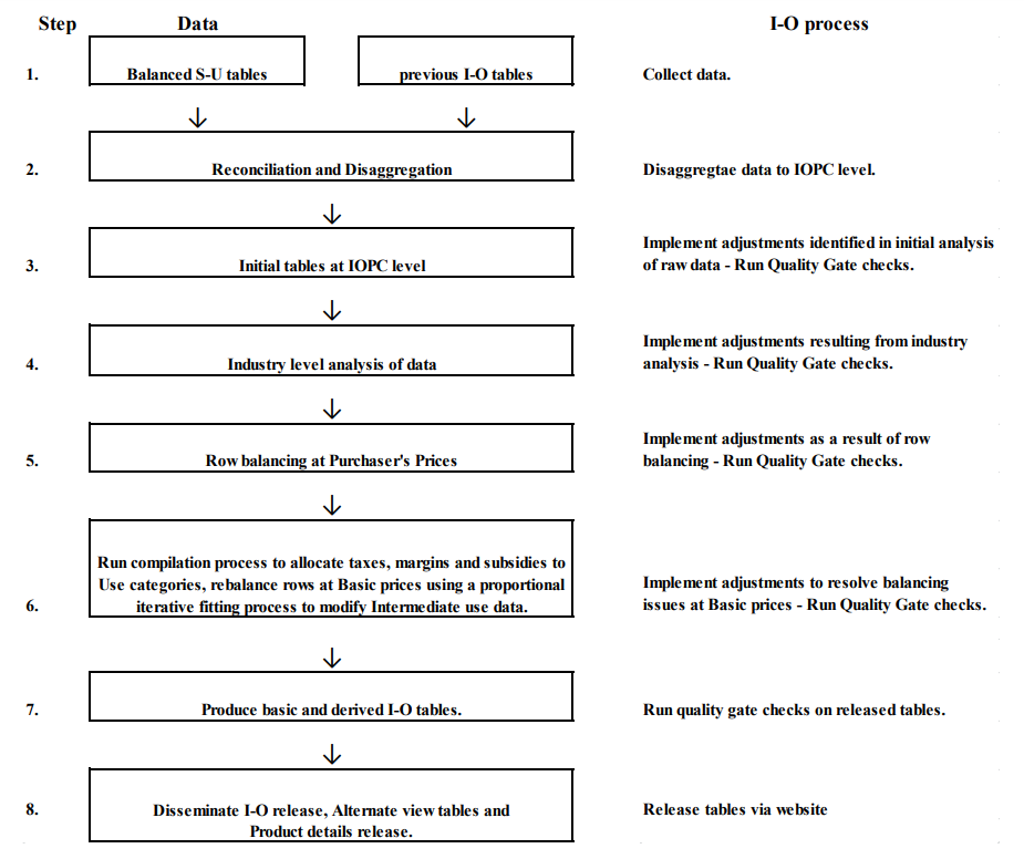
| Step | Data | I-O Process | |||||||
|---|---|---|---|---|---|---|---|---|---|
| 1 | Balanced S-U tables | Previous I-O tables | Collect data | ||||||
| ↓ | ↓ | ||||||||
| 2 | Reconcilation and Disaggregation | Disaggregate data to IPOC level | |||||||
| ↓ | |||||||||
| 3 | Initial tables at IOPC level | Implement adjustments identified in initial analysis of raw data - Run Quality Gate checks. | |||||||
| ↓ | |||||||||
| 4 | Industry level analysis of data | Implement adjustments resulting from industry analysis - Run Quality Gate checks. | |||||||
| ↓ | |||||||||
| 5 | Row balancing at Purchaser's Prices | Implement adjustments as a result of row balancing - Run Quality Gate checks. | |||||||
| ↓ | |||||||||
| 6 | Run compilation process to allocate taxes, margins and subsidies to Use categories, rebalance rows at Basic prices using a proportional iterative fitting process to modify Intermediate use of data. | Implement adjustments to resolve balancing issues at Basis prices - Run Quality Gate checks. | |||||||
| ↓ | |||||||||
| 7 | Produce basic and derived I-O tables | Run quality gate checks on released tables | |||||||
| ↓ | |||||||||
| 8 | Disseminate I-O release, Alternative view tables and Product details release. | Release tables via website | |||||||
Step 1: Collect source data
22.97 Obtain the S-U tables and previous I-O tables.
Step 2: Reconciliation and disaggregation
22.98 Balanced S-U tables are disaggregated in order to populate the I-O tables, ensuring consistency with the rest of national accounts published aggregates.
22.99 Much of the initial data used to populate the S-U tables is classified at the IOPC and IOIG levels, and then aggregated to the SUPC and SUIC levels. It is at this level that the balancing process of the S-U table is undertaken in order to produce balanced GDP estimates for the national accounts. It is necessary to then disaggregate the S-U products and industries to the I-O level in order to begin production of the I-O tables.
22.100 The disaggregation of the S-U level to the I-O level does not necessarily result in the same I-O distribution, compared with the initial I-O level data. This is due to the balancing being undertaken at the S-U level, and any adjustments made at that level may result in a different S-U level total than the initial total. This difference has to be distributed back to the I-O level and is done in several ways, depending on the component.
22.101 The following table outlines how the S-U level components are disaggregated to the I-O level.
| Industry | Supply | Intermediate consumption | |
|---|---|---|---|
| Agriculture, forestry and fishing | |||
| Agriculture | |||
| Economic Activity Survey ANZSIC class-level data are mapped to Input-Output Product Classifications using weights derived from Value of Agricultural Commodities Produced, Australia product data and previously published I-O weights. Any adjustments made during the S-U balancing process are split back to IOPCs based on the original IOPC proportions. | Intermediate consumption is disaggregated to the IOIG and IOPC level based on the final total intermediate use matrix from the previous year's I-O tables. | ||
| Forestry, aquaculture, fishing, hunting, trapping and services to agriculture, forestry and fishing | |||
| EAS ANZSIC class-level data are mapped directly to the primary Input-Output Product Groups. IOPG data are then mapped to IOPC using weights derived from previously published I-O data. Any adjustments made during the S-U balancing process are split back to IOPCs based on the original IOPC proportions. | Intermediate consumption is disaggregated to the IOIG and IOPC level based on the final total intermediate use matrix from the previous year's I-O tables. | ||
| Agriculture, forestry and fishing support services | |||
| EAS ANZSIC class-level data are mapped to primary Input-Output Product Groups. IOPG data are then mapped to IOPC using weights derived from previously published I-O data except for data supplied directly from source data at the IOPC level (e.g. ABARES ginned cotton). Any adjustments made during the SU balancing process are split back to IOPC based on the original IOPC proportions. | Intermediate consumption is disaggregated to the IOIG and IOPC level based on the final total intermediate use matrix from the previous year's I-O tables. | ||
| Mining | |||
| All except exploration and mining support services | |||
| State Mines product detail is mapped directly to IOPC. Any adjustments made during the S-U balancing process are split back to IOPCs based on the original IOPC proportions. | Intermediate consumption is disaggregated to the IOIG and IOPC level based on the final total intermediate use matrix from the previous year's I-O tables. | ||
| Exploration and mining support services | |||
| IOPC detail is a combination of EAS, Mineral Exploration and Petroleum Exploration data. Any adjustments made during the S-U balancing process are split back to IOPCs based on the original IOPC proportions. | Intermediate consumption is disaggregated to the IOIG and IOPC level based on the final total intermediate use matrix from the previous year's I-O tables. | ||
| Manufacturing | |||
| EAS ANZSIC class-level data are mapped to IOIGs and then split into primary IOPCs according to historical weights and the EAS data items. Any adjustments made during the S-U balancing process are split back to IOPCs based on the original IOPC proportions. | Intermediate consumption is disaggregated to the IOIG and IOPC level based on the final total intermediate use matrix from the previous year's I-O tables. | ||
| Electricity, gas, water and water services | |||
| EAS ANZSIC class-level data are mapped to IOIGs and then split into primary IOPCs according to historical weights and the EAS data items. Any adjustments made during the S-U balancing process are split back to IOPCs based on the original IOPC proportions. | Intermediate consumption is disaggregated to the IOIG and IOPC level based on the final total intermediate use matrix from the previous year's I-O tables. | ||
| Construction | |||
| EAS ANZSIC class-level data are mapped to IOIGs and then split into primary IOPCs according to historical weights adjusted for the movement in the Building Activity and Engineering Construction surveys. As the SUPC and IOPC are a one-to-one match, any adjustments made during the S-U balancing process are applied directly back to the IOPCs. | Intermediate consumption is disaggregated to the IOIG and IOPC level based on the final total intermediate use matrix from the previous year's I-O tables. | ||
| Wholesale trade | |||
| EAS ANZSIC class-level data are used to derive output which is mapped to IOPC based on historical proportions from previous retail and wholesale industry surveys and weights derived from previously balanced I-O tables. Any adjustments made during the S-U balancing process are split back to IOPCs based on the original IOPC proportions. | Intermediate consumption is disaggregated to the IOIG and IOPC level based on the final total intermediate use matrix from the previous year's I-O tables. | ||
| Retail trade | |||
| EAS ANZSIC class-level data are used to derive output which is mapped to IOPC based on historical proportions from previous retail and wholesale industry surveys and weights derived from previously balanced I-O tables. Any adjustments made during the S-U balancing are split back to the IOPCs based on the original IOPC proportions. | Intermediate consumption is disaggregated to the IOIG and IOPC level based on the final total intermediate use matrix from the previous year's I-O tables. | ||
| Accommodation and food services | |||
| EAS ANZSIC class-level data are mapped to primary IOPCs. Proportions are derived from ABS publications: Accommodation Services, Australia, Clubs, Pubs, Taverns and Bars, Australia and Cafes, Restaurants and Catering Services, Australia. Any adjustments made during the S-U balancing process are split back to IOPCs based on the original IOPC proportions. | Intermediate consumption is disaggregated to the IOIG and IOPC level based on the final total intermediate use matrix from the previous year's I-O tables. | ||
| Transport, postal and warehousing | |||
| EAS ANZSIC class-level data are mapped to IOIGs and then split into primary IOPCs according to historical weights. Any adjustments made during the S-U balancing process are split back to IOPCs based on the original IOPC proportions. | Intermediate consumption is disaggregated to the IOIG and IOPC level based on the final total intermediate use matrix from the previous year's I-O tables. | ||
| Information media and telecommunications | |||
| EAS ANZSIC class-level data are mapped to IOIGs and then split into primary IOPCs using previously balanced I-O tables weights. Any adjustments made during the S-U balancing process are split back to IOPCs based on the original IOPC proportions. | Intermediate consumption is disaggregated to the IOIG and IOPC level based on the final total intermediate use matrix from the previous year's I-O tables. | ||
| Financial and insurance services | |||
| Finance and Insurance and superannuation funds | |||
Data are compiled at the IOPC level. For details on the sources and methods used to compile finance and insurance and superannuation funds output data see Table 9.21 ANNUAL GROSS VALUE ADDED BY INDUSTRY—Finance services, subdivision 62 and Table 9.22 ANNUAL GROSS VALUE ADDED BY INDUSTRY—Insurance and superannuation funds, subdivision 63. Any adjustments made during the S-U balancing process are split back to IOPCs based on the original IOPC proportions. | Intermediate consumption is disaggregated to the IOIG and IOPC level based on the final total intermediate use matrix from the previous year's I-O tables. | ||
| Finance and insurance services | |||
| EAS ANZSIC class-level data are mapped to IOIGs and then split into primary IOPCs using weights from previously balanced I-O tables. Any adjustments made during the S-U balancing process are split back to IOPCs based on the original IOPC proportions. | Intermediate consumption is disaggregated to the IOIG and IOPC level based on the final total intermediate use matrix from the previous year's I-O tables. | ||
| Rental, hiring and real estate services, except ownership of dwellings | |||
| EAS ANZSIC class-level data are mapped to primary IOPCs according to historical weights. Any adjustments made during the S-U balancing process are split back to IOPCs based on the original IOPC proportions. | Intermediate consumption is disaggregated to the IOIG and IOPC level based on the final total intermediate use matrix from the previous year's I-O tables. | ||
| Professional, scientific and technical services | |||
| EAS ANZSIC class-level data are mapped to IOIGs and then split into primary IOPCs according to previous balanced I-O table weights. Any adjustments made during the S-U balancing process are split back to IOPCs based on the original IOPC proportions. | Intermediate consumption is disaggregated to the IOIG and IOPC level based on the final total intermediate use matrix from the previous year's I-O tables. | ||
| Administrative and supportive services | |||
| EAS ANZSIC class-level data are mapped to IOIGs and then split into primary IOPCs according to previous balanced I-O table weights. Any adjustments made during the S-U balancing process are split back to IOPCs based on the original IOPC proportions. | Intermediate consumption is disaggregated to the IOIG and IOPC level based on the final total intermediate use matrix from the previous year's I-O tables. | ||
| Public administration and safety | |||
| Government Finance Statistics gross expenditure data is classified according to the Classification of the Functions of Government - Australia. COFOG-A is mapped to the IOPC based on historical I-O weights and aggregated to the SUPC level. Any adjustments made during the S-U balancing process are split back to IOPCs based on the original IOPC proportions. | Intermediate consumption is disaggregated to the IOIG and IOPC level based on the final total intermediate use matrix from the previous year's I-O tables. | ||
| Education and training | |||
| Government Finance Statistics gross expenditure data is classified according to the Classification of the Functions of Government - Australia. COFOG-A is mapped to the IOPC based on historical I-O weights and aggregated to the SUPC level. ACARA and EAS ANZSIC class-level data are mapped to IOIGs and then split directly into primary IOPCs except for ANZSIC Class 8023 Combined primary and secondary education, which is split evenly between primary and secondary education services. Any adjustments made during the S-U balancing process are split back to IOPCs based on the original IOPC proportions. | Intermediate consumption is disaggregated to the IOIG and IOPC level based on the final total intermediate use matrix from the previous year's I-O tables. | ||
| Health care and social assistance | |||
| Supply is derived using the demand-side approach which sums the intermediate consumption of health and social assistance related products and final demand (i.e. final consumption expenditure, and exports less imports). These data are compiled at the IOPC level. Any adjustments made during the S-U balancing process are split back to IOPCs based on the original IOPC proportions. | Intermediate consumption is disaggregated to the IOIG and IOPC level based on the final total intermediate use matrix from the previous year's I-O tables. | ||
| Arts and recreation services | |||
| Arts and recreations services, except gambling | |||
| EAS data by ANZSIC Class level and institutional sector are mapped to primary IOPCs according to historical weights. Any adjustments made during the S-U balancing process are split back to IOPCs based on the original IOPC proportions. | Intermediate consumption is disaggregated to the IOIG and IOPC level based on the final total intermediate use matrix from the previous year's I-O tables. | ||
| Gambling | |||
| Supply is derived using the demand-side approach which sums the intermediate consumption of gambling products and final demand (i.e. final consumption expenditure, and exports less imports). These data are compiled at the IOPC level. Any adjustments made during the S-U balancing process are split back to IOPCs based on the original IOPC proportions. | Intermediate consumption is disaggregated to the IOIG and IOPC level based on the final total intermediate use matrix from the previous year's I-O tables. | ||
| Other services | |||
| Repairs and maintenance | |||
| EAS ANZSIC class-level data are mapped to IOIGs and then split into primary IOPCs according to historical weights and the EAS data items. Any adjustments made during the S-U balancing process are split back to IOPCs based on the original IOPC proportions. | Intermediate consumption is disaggregated to the IOIG and IOPC level based on the final total intermediate use matrix from the previous year's I-O tables. | ||
| Personal and other services | |||
| Supply is derived using the demand-side approach which sums the intermediate consumption of personal and other services products and final demand (i.e. final consumption expenditure, and exports less imports). These data are compiled at the IOPC level. Any adjustments made during the S-U balancing process are split back to IOPCs based on the original IOPC proportions. | Intermediate consumption is disaggregated to the IOIG and IOPC level based on the final total intermediate use matrix from the previous year's I-O tables. | ||
| Ownership of dwellings | |||
| Estimates for actual and imputed rental, consumption of fixed capital and trade data are all compiled at the IOPC level. The output of residential caravan parks is derived using the movement in service income from the EAS data for this ANZSIC class and applied to the estimate of the previous year. Any adjustments made during the S-U balancing process are split back to IOPCs based on the original IOPC proportions. | Intermediate consumption is disaggregated to the IOIG and IOPC level based on the final total intermediate use matrix from the previous year's I-O tables. | ||
| Taxes less subsidies on products | |||
Government Finance Statistics data classified by purpose and tax type are mapped to the I-O level using historical weights and other observed taxation statistics data. Data are compiled at the IOPC level and aggregated to SUPC for SU tables. Taxes are not adjusted during the S-U balancing process. | |||
| Trade and transport Margins | |||
| The most recent I-O Table’s distribution of margin by IOPC for each margin type is used to allocate each margin to a product. | |||
Changes made to classifications
From 03/04/2024 for Public administration and safety and Education and training, GFS gross expenditure data is classified according to the Classification of the Functions of Government- Australia (COFOG-A). Previously this publication stated that GFS data was classified according to the Government Purpose Classification (GPC).
For supply of Education and training, ACARA and EAS ANZSIC class-level data are mapped to IOIGs and then split directly into primary IOPCs. Previously only EAS ANZSIC class-level data was mapped to IOIGs.
Table 22.7 prior to 04/03/2024 update
| Item | Disaggregation method |
|---|---|
| Household final consumption expenditure | |
HFCE data are compiled according to the Classification of Individual Consumption by Purpose and is disaggregated to IOPC level based on balanced S-U table and previous year’s I-O table. Any adjustments made through the S-U balancing process are applied to the appropriate IOPC based on the intelligence for the decision. If detailed information is not known, it is allocated based on previously balanced I-O tables. | |
| Government final consumption expenditure | |
GFCE data are compiled according to the Classification of the Functions of Government - Australia , which is mapped to IOPC using historical input-output weights and aggregated for the S-U tables. Any adjustments made during the S-U balancing process are applied to the appropriate IOPC based on the intelligence for the decision. If detailed information is not known, it is allocated based on previous I-O tables. | |
| Gross fixed capital formation | |
GFCF data are compiled according to asset type by sector. With the exception of machinery and equipment, all asset types align with the IOPC. Machinery and equipment is disaggregated to the IOPC level based on previous years’ I-O tables, and converted into current-year prices using price indexes. Any adjustments applied during the balancing process are based on an informed assessment of how and why the imbalance has occurred. In cases where the required level of detail cannot be sourced, the allocation is based on previously-balanced I-O tables or the original proportions of the correspondence. | |
| Changes in inventories | |
| Changes in inventories is distributed across IOPCs based on how changes in inventories is distributed across IOPCs in the latest set of balanced I-O tables. | |
| Exports of goods and services | |
International trade data is mapped to the IOPC using the Australian Harmonised Export Commodity Classification (AHECC to IOPC correspondence). Further adjustments based on Balance of Payments data are made to the relevant IOPCs where appropriate. Further adjustments at the IOPC level may be required for product and industry balancing purposes. All such adjustments are offset to ensure that total exports remain unchanged. | |
| Imports of goods and services | |
International Trade data is mapped to the IOPC using the Harmonised Tariff Item Statistical Classification (HTISC to IOPC correspondence). Further adjustments based on Balance of Payments data are made to the relevant IOPCs where appropriate. Further adjustments at the IOPC level may be required for product and industry balancing purposes. All such adjustments are offset to ensure that total imports remain unchanged. | |
Changes made to classifications
From 03/04/2024 for Government final consumption expenditure, GFS gross expenditure data is classified according to the Classification of the Functions of Government- Australia (COFOG-A). Previously this publication stated that GFS data was classified according to the Government Purpose Classification (GPC).
Table 22.8 prior to 04/03/2024 update
| Industry/Item | Compensation of employees | Gross operating surplus/Gross mixed income | Other taxes less subsidies on production |
|---|---|---|---|
| Agriculture, forestry and fishing | |||
Data from the EAS are received at ANZSIC class level and then aggregated to IOIG. Data received at the ANZSIC division level (e.g. government data, payment in kind and fringe benefits tax) are disaggregated to IOIG level using proportions based on either general government output or EAS wages data as appropriate. Data are combined at the IOIG level initially and subsequently aggregated to SUIC. Any adjustments made during the S-U balancing process are disaggregated to the relevant IOIG level based on industry evidence. | Gross operating surplus/Gross mixed income (GOS/GMI) is derived differently depending on the sector. For the private non-financial corporations sector and unincorporated enterprises GOS/GMI is derived from the EAS data as a residual. GOS for NPISH units and general government units is equivalent to consumption of fixed capital. For more detail on the derivation of GOS/GMI refer to tables 11.5 to 11.10. Any adjustments made to GOS/GMI for the private non-financial corporations sector during S-U Table balancing process are allocated to IOIGs using IOIG proportions when originally compiled. | Data are compiled at the IOIG level and aggregated to the SUIC level for the S-U tables. Government Finance Statistics data is classified by purpose and tax type, which are then mapped to the IOPC level using historical weights and other observed taxation statistics data. | |
| Mining | |||
Data from the EAS are received at ANZSIC class level and then aggregated to IOIG. Data received at the ANZSIC division level (e.g. government data, payment in kind and fringe benefits tax) are disaggregated to IOIG level using proportions based on either general government output or EAS wages data as appropriate. Data are combined at the IOIG level initially and subsequently aggregated to SUIC. Any adjustments made during the S-U balancing process are disaggregated to the relevant IOIG based on industry evidence. | Gross operating surplus/Gross mixed income (GOS/GMI) is derived differently depending on the sector. For the private non-financial corporations sector and unincorporated enterprises GOS/GMI is derived from the EAS data as a residual. GOS for NPISH units and general government units is equivalent to consumption of fixed capital. For more detail on the derivation of GOS/GMI refer to tables 11.5 to 11.10. Any adjustments made to GOS/GMI for the private non-financial corporations sector during S-U Table balancing process are allocated to IOIGs using the output proportions. | Data are compiled at the IOIG level and aggregated to the SUIC level for the S-U tables. Government Finance Statistics data is classified by purpose and tax type which are then mapped to the IOPC level using historical weights and other observed taxation statistics data. | |
| Manufacturing | |||
Data from the EAS are received at ANZSIC class level and then aggregated to IOIG. Data received at the ANZSIC division level (e.g. government data, payment in kind and fringe benefits tax) are disaggregated to IOIG level using proportions based on either general government output or EAS wages data as appropriate. Data are combined at the IOIG level initially and subsequently aggregated to SUIC. Any adjustments made during the S-U balancing process are disaggregated to the relevant IOIG based on industry evidence. | Gross operating surplus/Gross mixed income (GOS/GMI) is derived differently depending on the sector. For the private non-financial corporations sector and unincorporated enterprises GOS/GMI is derived from the EAS data as a residual. GOS for NPISH units and general government units is equivalent to consumption of fixed capital. For more detail on the derivation of GOS/GMI refer to tables 11.5 to 11.10. Any adjustments made to GOS/GMI for the private non-financial corporations sector during the S-U Table balancing process are allocated to IOIGs using IOIG proportions from when originally compiled. | Data are compiled at the IOIG level and aggregated to the SUIC level for the S-U tables. Government Finance Statistics data is classified by purpose and tax type which are then mapped to the IOPC level using historical weights and other observed taxation statistics data. | |
| Electricity, gas, water and water services | |||
Data from the EAS are received at ANZSIC class level and then aggregated to IOIG. Data received at the ANZSIC division level (e.g. government data, payment in kind and fringe benefits tax) are disaggregated to IOIG level using proportions based on either general government output or EAS wages data as appropriate. Data are combined at the IOIG level initially and subsequently aggregated to SUIC. Any adjustments made during the S-U balancing process are disaggregated to the relevant IOIG based on industry evidence. | Gross operating surplus/Gross mixed income (GOS/GMI) is derived differently depending on the sector. For the private non-financial corporations sector and unincorporated enterprises GOS/GMI is derived from the EAS data as a residual. GOS for NPISH units and general government units is equivalent to consumption of fixed capital. For more detail on the derivation of GOS/GMI refer to tables 11.5 to 11.10. Any adjustments made to GOS/GMI for the private non-financial corporations sector during the S-U Table balancing process are allocated to IOIGs using IOIG proportions from when originally compiled. | Data are compiled at the IOIG level and aggregated to the SUIC level for the S-U tables. Government Finance Statistics data is classified by purpose and tax type which are then mapped to the IOPC level using historical weights and other observed taxation statistics data. | |
| Construction | |||
Data from the EAS are received at ANZSIC class level and then aggregated to IOIG. Data received at the ANZSIC division level (e.g. government data, payment in kind and fringe benefits tax) are disaggregated to IOIG level using proportions based on either general government output or EAS wages data as appropriate. Data are combined at the IOIG level initially and subsequently aggregated to SUIC. Any adjustments made during the S-U balancing process are disaggregated to the relevant IOIG based on industry evidence. | Gross operating surplus/Gross mixed income (GOS/GMI) is derived differently depending on the sector. For the private non-financial corporations sector and unincorporated enterprises GOS/GMI is derived from the EAS data as a residual. GOS for NPISH units and general government units is equivalent to consumption of fixed capital. For more detail on the derivation of GOS/GMI refer to tables 11.5 to 11.10. Any adjustments made to GOS/GMI for the private non-financial corporations sector during the S-U Table balancing process are allocated to IOIGs using IOIG proportions from when originally compiled. | Data are compiled at the IOIG level and aggregated to the SUIC level for the S-U tables. Government Finance Statistics data is classified by purpose and tax type which are then mapped to the IOPC level using historical weights and other observed taxation statistics data. | |
| Wholesale trade | |||
Data from the EAS are received at ANZSIC class level and then aggregated to IOIG. Data received at the ANZSIC division level (e.g. government data, payment in kind and fringe benefits tax) are disaggregated to IOIG level using proportions based on either general government output or EAS wages data as appropriate. Data are combined at the IOIG level initially and subsequently aggregated to SUIC. Any adjustments made during the S-U balancing process are disaggregated to the relevant IOIG based on industry evidence. | Gross operating surplus/Gross mixed income (GOS/GMI) is derived differently depending on the sector. For the private non-financial corporations sector and unincorporated enterprises GOS/GMI is derived from the EAS data as a residual. GOS for NPISH units and general government units is equivalent to consumption of fixed capital. For more detail on the derivation of GOS/GMI refer to tables 11.5 to 11.10. Any adjustments made to GOS/GMI for the private non-financial corporations sector during S-U Table balancing process are allocated to IOIGs directly as SUICs and IOIGs have a one-to-one relationship. | Data are compiled at the IOIG level and aggregated to the SUIC level for the S-U tables. Government Finance Statistics data is classified by purpose and tax type which are then mapped to the IOPC level using historical weights and other observed taxation statistics data. | |
| Retail trade | |||
Data from the EAS are received at ANZSIC class level and then aggregated to IOIG. Data received at the ANZSIC division level (e.g. government data, payment in kind and fringe benefits tax) are disaggregated to IOIG level using proportions based on either general government output or EAS wages data as appropriate. Data are combined at the IOIG level initially and subsequently aggregated to SUIC. Any adjustments made during the S-U balancing process are disaggregated to the relevant IOIG based on industry evidence. | Gross operating surplus/Gross mixed income (GOS/GMI) is derived differently depending on the sector. For the private non-financial corporations sector and unincorporated enterprises GOS/GMI is derived from the EAS data as a residual. GOS for NPISH units and general government units is equivalent to consumption of fixed capital. For more detail on the derivation of GOS/GMI refer to tables 11.5 to 11.10. Any adjustments made to GOS/GMI for the private non-financial corporations sector during S-U Table balancing process are allocated to IOIGs directly as SUICs and IOIGs have a one-to-one relationship. | Data are compiled at the IOIG level and aggregated to the SUIC level for the S-U tables. Government Finance Statistics data is classified by purpose and tax type which are then mapped to the IOPC level using historical weights and other observed taxation statistics data. | |
| Accommodation and food services | |||
Data from the EAS are received at ANZSIC class level and then aggregated to IOIG. Data received at the ANZSIC division level (e.g. government data, payment in kind and fringe benefits tax) are disaggregated to IOIG level using proportions based on either general government output or EAS wages data as appropriate. Data are combined at the IOIG level initially and subsequently aggregated to SUIC. Any adjustments made during the S-U balancing process are disaggregated to the relevant IOIG based on industry evidence. | Gross operating surplus/Gross mixed income (GOS/GMI) is derived differently depending on the sector. For the private non-financial corporations sector and unincorporated enterprises GOS/GMI is derived from the EAS data as a residual. GOS for NPISH units and general government units is equivalent to consumption of fixed capital. For more detail on the derivation of GOS/GMI refer to tables 11.5 to 11.10. Any adjustments made to GOS/GMI for the private non-financial corporations sector during S-U Table balancing process are allocated to IOIGs directly as SUICs and IOIGs have a one-to-one relationship. | Data are compiled at the IOIG level and aggregated to the SUIC level for the S-U tables. Government Finance Statistics data is classified by purpose and tax type which are then mapped to the IOPC level using historical weights and other observed taxation statistics data. | |
| Transport, postal and warehousing | |||
Data from the EAS are received at ANZSIC class level and then aggregated to IOIG. Data received at the ANZSIC division level (e.g. government data, payment in kind and fringe benefits tax) are disaggregated to IOIG level using proportions based on either general government output or EAS wages data as appropriate. Data are combined at the IOIG level initially and subsequently aggregated to SUIC. Any adjustments made during the S-U balancing process are disaggregated to the relevant IOIG based on industry evidence. | Gross operating surplus/Gross mixed income (GOS/GMI) is derived differently depending on the sector. For the private non-financial corporations sector and unincorporated enterprises GOS/GMI is derived from the EAS data as a residual. GOS for NPISH units and general government units is equivalent to consumption of fixed capital. For more detail on the derivation of GOS/GMI refer to tables 11.5 to 11.10. Any adjustments made to GOS/GMI for the private non-financial corporations sector during the S-U Table balancing process are allocated to IOIGs using IOIG proportions from when originally compiled. | Data are compiled at the IOIG level and aggregated to the SUIC level for the S-U tables. Government Finance Statistics data is classified by purpose and tax type which are then mapped to the IOPC level using historical weights and other observed taxation statistics data. | |
| Information media and telecommunications | |||
Data from the EAS are received at ANZSIC class level and then aggregated to IOIG. Data received at the ANZSIC division level (e.g. government data, payment in kind and fringe benefits tax) are disaggregated to IOIG level using proportions based on either general government output or EAS wages data as appropriate. Data are combined at the IOIG level initially and subsequently aggregated to SUIC. Any adjustments made during the S-U balancing process are disaggregated to the relevant IOIG based on industry evidence. | Gross operating surplus/Gross mixed income (GOS/GMI) is derived differently depending on the sector. For the private non-financial corporations sector and unincorporated enterprises GOS/GMI is derived from the EAS data as a residual. GOS for NPISH units and general government units is equivalent to consumption of fixed capital. For more detail on the derivation of GOS/GMI refer to tables 11.5 to 11.10. Any adjustments made to GOS/GMI for the private non-financial corporations sector during S-U Table balancing process are allocated to IOIGs directly as SUICs and IOIGs have a one-to-one relationship. | Data are compiled at the IOIG level and aggregated to the SUIC level for the S-U tables. Government Finance Statistics data is classified by purpose and tax type which are then mapped to the IOPC level using historical weights and other observed taxation statistics data. | |
| Financial and insurance services | |||
There is a one-to-one mapping between the IOIG and SUIC for this industry. This means that movements at the IOIG level are consistent with those in the S-U table benchmarks. Tables 11.1 and 11.2 provide details on the sources and methods used to compile COE for financial corporations. | For SUIC 620 Finance and SUIC 630 Insurance and Superannuation Funds, GOS is compiled from source data at IOIG level. For SUIC 640 Auxiliary Finance and Insurance Services, GOS is derived as a residual item from EAS data, also at the IOIG level. For more detail on the derivation of GOS/GMI refer to tables 11.5 to 11.10. | Data are compiled at the IOIG level and aggregated to the SUIC level for the S-U tables. Government Finance Statistics data is classified by purpose and tax type which are then mapped to the IOPC level using historical weights and other observed taxation statistics data. | |
| Rental, hiring and real estate services, except ownership of dwellings | |||
Data from the EAS are received at ANZSIC class level and then aggregated to IOIG. Data received at the ANZSIC division level (e.g. government data, payment in kind and fringe benefits tax) are disaggregated to IOIG level using proportions based on either general government output or EAS wages data as appropriate. Data are combined at the IOIG level initially and subsequently aggregated to SUIC. Any adjustments made during the S-U balancing process are disaggregated to the relevant IOIG based on industry evidence. | Gross operating surplus/Gross mixed income (GOS/GMI) is derived differently depending on the sector. For the private non-financial corporations sector and unincorporated enterprises GOS/GMI is derived from the EAS data as a residual. GOS for NPISH units and general government units is equivalent to consumption of fixed capital. For more detail on the derivation of GOS/GMI refer to tables 11.5 to 11.10. Any adjustments made to GOS/GMI for the private non-financial corporations sector during S-U Table balancing process are allocated to IOIGs directly as SUICs and IOIGs have a one-to-one relationship. | Data are compiled at the IOIG level and aggregated to the SUIC level for the S-U tables. Government Finance Statistics data is classified by purpose and tax type which are then mapped to the IOPC level using historical weights and other observed taxation statistics data. | |
| Professional, scientific and technical services | |||
Data from the EAS are received at ANZSIC class level and then aggregated to IOIG. Data received at the ANZSIC division level (e.g. government data, payment in kind and fringe benefits tax) are disaggregated to IOIG level using proportions based on either general government output or EAS wages data as appropriate. Data are combined at the IOIG level initially and subsequently aggregated to SUIC. Any adjustments made during the S-U balancing process are disaggregated to the relevant IOIG based on industry evidence. | Gross operating surplus/Gross mixed income (GOS/GMI) is derived differently depending on the sector. For the private non-financial corporations sector and unincorporated enterprises GOS/GMI is derived from the EAS data as a residual. GOS for NPISH units and general government units is equivalent to consumption of fixed capital. For more detail on the derivation of GOS/GMI refer to tables 11.5 to 11.10. Any adjustments made to GOS/GMI for the private non-financial corporations sector during S-U Table balancing process are allocated to IOIGs directly as SUICs and IOIGs have a one-to-one relationship. | Data are compiled at the IOIG level and aggregated to the SUIC level for the S-U tables. Government Finance Statistics data is classified by purpose and tax type which are then mapped to the IOPC level using historical weights and other observed taxation statistics data. | |
| Administrative and supportive services | |||
Data from the EAS are received at ANZSIC class level and then aggregated to IOIG. Data received at the ANZSIC Division level (e.g. government data, payment in kind and fringe benefits tax) are disaggregated to IOIG level using proportions based on either general government output or EAS wages data as appropriate. Data are combined at the IOIG level initially and subsequently aggregated to SUIC. Any adjustments made during the S-U balancing process are disaggregated to the relevant IOIG based on industry evidence. | Gross operating surplus/Gross mixed income (GOS/GMI) is derived differently depending on the sector. For the private non-financial corporations sector and unincorporated enterprises GOS/GMI is derived from the EAS data as a residual. GOS for NPISH units and general government units is equivalent to consumption of fixed capital. For more detail on the derivation of GOS/GMI refer to tables 11.5 to 11.10. Any adjustments made to GOS/GMI for the private non-financial corporations and unincorporated enterprises during S-U Table balancing process are allocated to IOIGs using IOIG proportions when originally compiled. | Data are compiled at the IOIG level and aggregated to the SUIC level for the S-U tables. Government Finance Statistics data is classified by purpose and tax type which are then mapped to the IOPC level using historical weights and other observed taxation statistics data. | |
| Public administration and safety | |||
For SUIC 750 Government administration and regulatory services and 770 Public Order and Safety, data from the EAS are received at ANZSIC class level and then aggregated to IOIG. Government data are received at the ANZSIC division level and are disaggregated between these two IOIGs using their proportions of general government output. For SUIC 760 Defence, defence wages and salaries are mapped directly to this IOIG. Other data received or calculated at an ANZSIC division level (e.g. payment in kind and Fringe Benefits Tax) are disaggregated to IOIG level using either general government output or EAS wages data as appropriate. Data are combined at the IOIG level initially and subsequently aggregated to SUIC. | General government GOS is equivalent to the value of consumption of fixed capital on general government assets as derived in the Perpetual Inventory Method. This division contains minimal private non-financial corporations GOS. It is derived directly from EAS ANZSIC class-level data. For more detail on the derivation of GOS/GMI refer to tables 11.5 to 11.10. Any adjustments made to GOS/GMI for the private non-financial corporations sector during S-U Table balancing process are allocated to IOIGs directly as SUICs and IOIGs have a one-to-one relationship. | Data are compiled at the IOIG level and aggregated to the SUIC level for the S-U tables. Government Finance Statistics data is classified by purpose and tax type which are then mapped to the IOPC level using historical weights and other observed taxation statistics data. | |
| Education and training | |||
Data from the EAS are received at ANZSIC class level and then aggregated to IOIG. Data received at the ANZSIC division level (e.g. government data, payment in kind and fringe benefits tax) are disaggregated to IOIG level using proportions based on either general government output or EAS wages data as appropriate. Data are combined at the IOIG level initially and subsequently aggregated to SUIC. Any adjustments made during the S-U balancing process are disaggregated to the relevant IOIG based on industry evidence. | Gross operating surplus/Gross mixed income (GOS/GMI) is derived differently depending on the sector. For the private non-financial corporations sector and unincorporated enterprises GOS/GMI is derived from the EAS data as a residual. GOS for NPISH units and general government units is equivalent to consumption of fixed capital. For more detail on the derivation of GOS/GMI refer to tables 11.5 to 11.10. Any adjustments made to GOS/GMI for the private non-financial corporations sector during S-U Table balancing process are allocated to IOIGs directly as SUICs and IOIGs have a one-to-one relationship. | Data are compiled at the IOIG level and aggregated to the SUIC level for the S-U tables. Government Finance Statistics data is classified by purpose and tax type which are then mapped to the IOPC level using historical weights and other observed taxation statistics data. | |
| Health care and social assistance | |||
Data from the EAS are received at ANZSIC class level and then aggregated to IOIG. Data received at the ANZSIC division level (e.g. government data, payment in kind and fringe benefits tax) are disaggregated to IOIG level using proportions based on either general government output or EAS wages data as appropriate. Data are combined at the IOIG level initially and subsequently aggregated to SUIC. Any adjustments made during the S-U balancing process are disaggregated to the relevant IOIG based on industry evidence. | Gross operating surplus (GOS) and gross mixed income is taken from 5204.0 (Total Factor Income by Industry and principal components – Current prices) at division level. General Government GOS is subtracted from the division level GOS/GMI to derive private GOS/GMI for the division. Private GOS/GMI for the division is then split by ratios based on the General Government GOS at IOIG level Any adjustments made to GOS private during S-U Table balancing are allocated to IOIGs using IOIG proportions when originally compiled. | Data are compiled at the IOIG level and aggregated to the SUIC level for the S-U tables. Government Finance Statistics data is classified by purpose and tax type which are then mapped to the IOPC level using historical weights and other observed taxation statistics data. | |
| Arts and recreation services | |||
Data from the EAS are received at ANZSIC class level and then aggregated to IOIG. Data received at the ANZSIC division level (e.g. government data, payment in kind and fringe benefits tax) are disaggregated to IOIG level using proportions based on either general government output or EAS wages data as appropriate. Data are combined at the IOIG level initially and subsequently aggregated to SUIC.
Any adjustments made during the S-U balancing process are disaggregated to the relevant IOIG based on industry evidence. | For the Arts and recreation services division (except Gambling), gross operating surplus/gross mixed income (GOS/GMI) is derived differently depending on the sector. For the private non-financial corporations sector and unincorporated enterprises GOS/GMI is derived from the EAS data as a residual. GOS for NPISH units and general government units is equivalent to consumption of fixed capital. For more detail on the derivation of GOS/GMI refer to tables 11.5 to 11.10. For IOIG 9201 Gambling, gross operating surplus (GOS) and gross mixed income (GMI) is taken from 5204.0 (Total Factor Income by industry and principal components - Current prices) at division level. General Government GOS is subtracted from this to derive private GOS/GMI for the division. Private GOS/GMI by IOIG is then calculated from the division total using supply ratios. Any adjustments made to GOS/GMI for private non-financial corporations and unincorporated enterprises during S-U Table balancing process are allocated to IOIGs automatically as the SUICs and IOIGs have a one-to-one relationship. | Data are compiled at the IOIG level and aggregated to the SUIC level for the S-U tables. Government Finance Statistics data is classified by purpose and tax type which are then mapped to the IOPC level using historical weights and other observed taxation statistics data. | |
| Other services | |||
Data from the EAS are received at ANZSIC class level and then aggregated to IOIG. Data received at the ANZSIC division level (e.g. government data, payment in kind and fringe benefits tax) are disaggregated to IOIG level using proportions based on either general government output or EAS wages data as appropriate. Data are combined at the IOIG level initially and subsequently aggregated to SUIC.
Any adjustments made during the S-U balancing process are disaggregated to the relevant IOIG based on industry evidence. | For SUIC 940 Repair and Maintenance, gross operating surplus/gross mixed income (GOS/GMI) is derived differently depending on the sector. For the private non-financial corporations sector and unincorporated enterprises GOS/GMI is derived from the EAS data as a residual. GOS for NPISH units and general government units is equivalent to consumption of fixed capital. For more detail on the derivation of GOS/GMI refer to tables 11.5 to 11.10. Any adjustments made to GOS/GMI for the private non-financial corporations sector during S-U Table balancing process are allocated to IOIGs using IOIG proportions when originally compiled. For SUIC 950 Personal and Other Services, GOS for private non-financial corporations is compiled at SUIC level from EAS and COFC data, and disaggregated to IOIGs using historic weights. For more detail on the derivation of GOS/GMI refer to tables 11.5 to 11.10. Any adjustments made to GOS/GMI for private non-financial corporations and unincorporated enterprises during S-U Table balancing process are allocated to IOIGs using IOIG proportions when originally compiled. | Data are compiled at the IOIG level and aggregated to the SUIC level for the S-U tables. Government Finance Statistics data is classified by purpose and tax type which are then mapped to the IOPC level using historical weights and other observed taxation statistics data. | |
| Ownership of dwellings | |||
GOS is derived as a residual at the IOIG level. For more detail on the derivation of GOS/GMI refer to tables 11.5 to 11.10. This S-U Industry and IOIG have a one-to-one relationship therefore any adjustments made to GOS during S-U Table balancing process are allocated to the IOIG automatically. | |||
22.102 Once the disaggregation is completed it is necessary to reconcile (or confront) these results with additional information to ensure the distribution is coherent. The data sources, in addition to the main data sources used to compile the S-U tables, used in this reconciliation process are obtained from the following:
- ABS data:
- Australian Industry Statistics case study data;
- Value of Agricultural Commodities Produced data;
- Mineral and Petroleum Exploration data;
- Retail Trade;
- Quarterly Business Indicators;
- Building Approvals data;
- Engineering Construction data;
- Private Sector Construction data;
- Water Account data;
- Motor Vehicle Use data;
- Tourist Accommodation data;
- Household Expenditure data; and
- occasional publications;
- Office of the Chief Economist;
- Australian Bureau of Agricultural Resource Economics and Sciences:
- Agricultural Commodities; and
- Australian Forest and Wood Products Statistics;
- Department of Climate Change, Energy, the Environment and Water:
- Australian Petroleum Statistics;
- State departments of primary industries;
- Australian Prudential Regulatory Authority;
- Reserve Bank of Australia;
- Australian Taxation Office;
- Medicare statistics;
- annual reports;
- press and internet articles;
- private industry analysis; and
- industry body commentary.
22.103 The level of detail used in the disaggregation and reconciliation processes will vary depending on the component and its data source. The aim is to use the most detailed information where available. For example, detailed information is available at the IOPC level for international trade in goods statistics. However, IOPC level detail is not available for international trade in services or Government Finance Statistics. In this case, weights from the previous year’s I-O tables are applied to derive I-O estimates.
22.104 The disaggregation (and reconciliation) process will result in imbalances at the I-O levels. These imbalances are resolved during the balancing process described in the steps that follow.
Step 3: Alignment with the ASNA
22.105 The initial data at IOPC level is reviewed against quality measures (see next section for more details). This initial data quality assessment is designed to ensure that I-O estimates are fully aligned with the Australian System of National Accounts available at the time that the I-O tables are compiled.
22.106 Given the importance of margins in the I-O framework, detailed ratio analysis are undertaken to review the product allocation of trade margins.
22.107 Adjustments are implemented where required.
Step 4: Industry level analysis
22.108 The I-O tables are assessed against the quality measures via an industry view and adjustments made where necessary. The industry view assesses Australian production of products by each industry and the use of each product by other industries as part of the production process.
Step 5: Row balancing at purchasers’ prices
22.109 The supply of each product is balanced against the intermediate and final use of the product by a manual process using the data sources listed in step 2 above.
22.110 A principal edit undertaken in the compilation of I-O tables is to reconcile the flow of products through the productive process. Backward linkages are reconciled to ensure the process of products through the productive process is logical. For example, the Australian production of raw milk is compared to the intermediate use of products produced by the dairy manufacturing industry in milk and dairy product production. As a product is transformed or processed, the value of output should increase due to the increase in value added.
22.111 When all products are balanced at purchasers’ prices (PP), the data are assessed against the quality measures and adjustments made where required.
Step 6: Allocation of margins, taxes and subsidies and derivation of the Basic Price
22.112 Once the I-O tables are manually balanced at purchasers' prices (PP), the use categories at basic prices (BP) are modelled using the basic relationship PP = BP + MTS where MTS represents Margins, Taxes and Subsidies on products.
22.113 The disposition of each margin, tax or subsidy across the use categories is driven by a number of general rules. These rules are applied to all products except those with specific characteristics (see below) in order to ensure the resulting disposition of MTS is logical and coherent. In the use categories, for example, the retail margins can only be allocated to HFCE while wholesale margins can be allocated to all use categories (including intermediate use) except GFCE and inventories.
22.114 In a number of instances, the standard disposition of MTS is overwritten by special rules. These special rules are applied to products with specific use characteristics and ensure a better allocation of MTS for these products. An example of a special rule relates to goods consumed by tourists which can attract retail margins in exports.
22.115 Margins, taxes and subsidies are independently allocated across the use categories on a proportional basis according to the general and special rules. The total MTS by product is therefore allocated to all use categories for each product, first using the PP and then on BP once derived.
22.116 The BP is derived from the PP by subtracting MTS in intermediate use and final use. Because MTS are allocated independently, the resulting BP tables are unbalanced. A constrained optimisation process is used, once large imbalances have been resolved manually, to balance products and industries in the intermediate use matrix.
22.117 The different margins, taxes and subsidies are added to the BP in a cumulative manner. In most cases, transport margins will be applied before wholesale margins which will themselves be applied before retail margins. For practical reasons the incremental disposition of MTS is not applied but the basic price is assumed to be a better allocator for MTS. This is particularly true for products attracting a lot of retail margins and for which the inclusion of these margins would distort the disposition of other MTS.
22.118 Once derived, the BP is used to allocate MTS across the use categories. Manual adjustments are made where required. This process is repeated twice in order to gradually refine the disposition of MTS and the resulting BP.
22.119 When all products are balanced at BP the data are assessed against the quality measures and adjustments made where required.
Step 7: Produce basic and derived I-O tables
22.120 The next step is to produce basic and derived I-O tables. Quality checks are again run to assess data quality, and to check that publication standards have been applied to the tables for release.
22.121 The SNA68 transport margin adjustment is made (see section on the SNA68 transport margin adjustment at beginning of this chapter).
22.122 The alternate view tables are then prepared. The treatment applied to compile the alternate view removes the negative effect of the c.i.f./f.o.b. adjustment in imports (see section on c.i.f./f.o.b. adjustment for details).
22.123 The product details tables are then prepared.
22.124 All tables for release are assessed against quality measures and any corrections made as required.
Step 8: Disseminate I-O tables, alternate view tables and product details publication
22.125 Publication tables are disseminated on the ABS website. The last quality check is run to review the publication production cycle, and to identify and document improvements for the following cycle
Quality measures
22.126 Twenty quality measures are applied at the various steps in the compilation process described above. The quality measures include internal consistency checks and checks for consistency with published national account aggregates. Most of the quality measures are assessed at every gate with a few exceptions. The complete list of quality measures include:
- all three measures of GDP are equal when aggregated from the I-O tables;
- supply matches use in all rows (after product balancing);
- application of the SNA68 TMA does not affect PP overall estimates;
- the latest appropriate data for the reference period has been used;
- there are no negative values in supply;
- estimates match published estimates in the Australian National Accounts for the relevant reference period;
- known problems from previous I-O cycles have been resolved;
- c.i.f./f.o.b. adjustments have been applied correctly;
- there are no inventories of services and no margins attributed to services products;
- GST and retail margins are consistent with HFCE;
- domestic exports do not exceed production unless stock is drawn from Inventories;
- re-exports do not exceed imports unless stock is drawn from Inventories;
- coverage and specialisation ratios are sensible and consistent with previous I-O tables;
- supply is consistent with use for top 50 IOPCs;
- the COE/TIU and GOS/TIU ratios are plausible;
- inventory levels are sensible in relation to supply at basic prices;
- distribution of supply confronted with previous cycle is plausible;
- distribution of retail and wholesale margins is coherent;
- supply and final use column totals have not been changed; and
- issues identified at previous steps have been addressed.
\(\)
Using I-O tables for analysis
22.127 The basic tables and the industry-by-industry tables are an accounting record of the flows in the economy for a given year. If simplifying assumptions are used, the I-O tables can serve many analytical purposes. For example, it is possible to:
- estimate the levels of output of the production required to meet a given level of final demand;
- the effect of other industries of an additional output of $100m of a product; or
- the impact of additional exports of a product on other industries, by assuming the average and marginal utilisation rates are the same.
22.128 An impact analysis like this can be concerned with one or several industries in the economy, and can be done using the requirements table.
22.129 Relative prices are constantly changing, and do change significantly from year to year. It is useful to regard I-O tables as representing underlying quantities and technological relationships, rather than values and value relationships. Even factor payments (COE, GOS and GMI) can be viewed as representing quantities of employee services, and of entrepreneurial and capital services. Unless the analyst makes allowance for price changes, all proportions and values will be in terms of relative and absolute prices of the reference year.
22.130 The ABS I-O tables are not revised. They provide a snapshot of the Australian economy at a point-in-time and should not be used as time series.
Direct requirements coefficients
22.131 A simple application of the I-O tables is calculating inputs as a percentage of the output of an industry and using these percentages for estimating the input requirements for a given output of the industry. In all tables in the I-O releases, 100 always represents total Australian production, including tables with indirect allocation of imports.
22.132 All coefficients in the requirements matrices relate to flows from industry to industry. The application of the requirements will be in terms of the output of industries, and not of the products primary to the industries.
22.133 Direct requirements coefficients have different meanings depending on the treatment of imports in the flow table from which they are derived. If the flow table is based upon direct allocation of competing imports, the coefficients in quadrant 1 will only refer to the requirements from domestic production. If the flow tables are based upon an indirect allocation of imports, the coefficients in quadrant 1 will include the use of both imported and domestically produced products. If the usage of a product by an industry remains unchanged, substitution can take place between imports and domestic production without affecting the size of the coefficients.
22.134 The coefficients for COE, GOS and GMI, net taxes on products and other taxes on production are the same regardless of the allocation of imports in the source flow table. However, the coefficients for imports depend on the two types of table. In the tables with an indirect allocation of imports, the entries in quadrant 3 (the primary inputs quadrant) relate only to complementary imports (of which none are identified in current I-O tables), and competing imports are included in quadrant 1 since this shows the requirements of any given industry for the output of other industries and competing imports primary to those industries. In tables with a direct allocation of competing imports, the imports entries relate to all imports used by the industry.
Total requirements coefficients
22.135 The chain of calculations for output requirements can be continued beyond the direct requirements for an industry. For example, in order to produce output from the chemicals industry, inputs are required directly from the mining industry and other industries. To supply this direct requirement, the mining industry itself requires inputs from other industries including the chemicals industry, and so on in a convergent infinite series. In another example, the mining industry may not directly require inputs from agriculture but requires inputs from chemicals which cannot be produced without inputs from agriculture. Therefore, mining has an indirect requirement for input from agriculture. As is the case with the direct requirements coefficients, coefficients in the requirements matrices relate to flows from industry to industry. The application of the requirements will be in terms of the output of industries and not of the products primary to the industries.
22.136 The requirements can be traced, step by step through the industrial structure until the increments of output required indirectly for each industry become insignificant. This occurs after a few rounds. If this is done for all industries, and the direct and indirect requirements are added together, the result is a matrix of total requirements. However, if the number of industries is large the iterative process is too cumbersome, and the matrix is calculated by matrix inversion. This is why the matrix of total requirements is often referred to as the inverse matrix or Leontief inverse, and its coefficients as inverse coefficients.
22.137 In the total requirements coefficients table, at the intersection of a typical row i and column j, represents the units of output of industry i required directly and indirectly to produce 100 units of output absorbed by final demand of industry j. The tables are compiled based upon the assumptions of homogeneity and proportionality and this must be accounted for when they are used.
22.138 Derived coefficients will differ according to the way imports have been treated in the flow table from which they are derived. If competing imports were directly allocated in the flow table, the resultant total requirements coefficients in quadrant 1 will only refer to the requirements for domestic production. Therefore, when using of the coefficients it would be necessary to assume unchanged usage of imports or to regulate the coefficients by using revised import usage characteristics.
22.139 If the total requirements coefficients were derived from a flow table using indirect allocation of imports, the coefficients in quadrant 1 will be based on the usage of domestically produced and imported goods. If the usage of a product by an industry remains unchanged, substitution can therefore take place between domestic products and imports without affecting the size of the coefficients. In using the coefficients, an assessment of the proportion of the requirements that is likely to be satisfied by imports would need to be made, unless all demand can be met from Australian production.
22.140 All tables of total requirements characteristically have a diagonal entry that exceeds 100. The amounts that exceed 100 are due to the indirect requirements affecting each industry through other industries. This means that to meet 100 units of final demand for the output of an industry, the industry itself has to produce those 100 units, plus any direct or indirect requirements for its output resulting from requirements from itself, or from other industries.
Specially derived tables
22.141 Instead of being expressed as total output the requirements can be expressed as primary input content. This assumes that the final output of an industry is equal to the reward paid to the factors of production in all industries contributing directly and indirectly to this final output.
22.142 Each entry in the requirements table represents the total output required from the industry in the row, by the industry in the column for the purpose of producing $100 of output absorbed by final demand. Each of these can also be thought the sum of its inputs and can be dissected into its individual components. The proportions obtained from the column of the supplying industry in the table of direct coefficients are used. According to the proportionality assumption, the amount of each kind of input used by an industry represents a fixed proportion of the industries output.
Stability of I-O coefficients
22.143 The use of coefficients in users’ analyses will be accurate to the extent that the coefficients remain stable, which is dependent on the extent to which the assumptions of homogeneity and proportionality are valid.
22.144 The homogeneity assumption expresses that: each industry produces a single output (all products are perfect substitutes for one another, or are produced in fixed proportions); each industry has a single input structure (which does not vary in response to product mix); and there is no substitution between products of different groups. This assumption is weakened as product mixes change (with corresponding changes in input mixes), introduction of new products or materials, and as there is substitution between domestic production and imports or vice versa.
22.145 The proportionality assumption says that for any level of output the inputs will be a fixed proportion of the total. This assumption holds in the reference year but less so in each following year. The assumption may be invalidated by economies of scale, technological change, or substitution between the factors of production.
22.146 The I-O tables produced by the ABS represent an open I-O system as the final demand categories are exogenous (i.e. determined outside the system). In a closed system, all categories are defined as interdependent. For example, HFCE is treated like an industry, and its inputs (the requirements of consumers) are part of the solution. The ABS I-O tables are static as they provide a snapshot at a point-of-time. Dynamic systems introduce explicit time periods into the model and allow the change from a base period to the target to be traced.
Multipliers
22.147 Multipliers are a tool used by I-O practitioners to answer "what-if?" type questions. For example, 'what would be the impact on employment of a change in the output of the Chemicals manufacturing industry?' Multipliers can be used to quantify the flow-on effect of a change in the output of an industry on one or more of imports, income, employment or output on individual industries, or in total. The multipliers can be used to show "first-round" changes, or the aggregate effects once secondary effects have flowed through the system.
22.148 The ABS has published an information paper, Australian National Accounts: Introduction to Input-Output Multipliers, 1989-90, which provides a guide to the construction, interpretation and use of I-O multipliers.
22.149 The ABS published multipliers until the 1998-99 issue of Australian National Accounts: Input-Output Tables as Table 22. Production of multipliers was discontinued for several reasons. There was considerable debate in the user community as to their suitability for the purposes to which they were most commonly applied; that is, to produce measures of the size and impact of a particular project to support bids for industry assistance of various forms.
22.150 The ABS frequently receives requests from users who are seeking updated Input-Output multipliers. It is currently unable to support user requests for assistance with multipliers, and does not plan to compile and reissue this table. For this reason, Table 22 is missing from the list of basic tables published by the ABS at the beginning of this chapter.
Limitations of Input-Output Multipliers for Economic Impact Assessment
22.151 I-O multipliers are most commonly used to quantify the economic impacts (both direct and indirect) relating to policies and projects. While their ease of use makes I-O multipliers a popular tool for economic impact analysis, they are based on limiting assumptions that results in multipliers being a biased estimator of the benefits or costs of a project.
22.152 Inherent shortcomings and limitations of multipliers for economic impact analysis include:
- Lack of supply-side constraints – the most significant limitation of economic impact analysis using multipliers is the implicit assumption that the economy has no supply-side constraints. That is, it is assumed that extra output can be produced in one area without taking away resources from other activities, thus overstating economic impacts. The actual impact is likely to be dependent on the extent to which the economy is operating at or near capacity.
- Fixed prices – constraints on the availability of inputs, such as skilled labour, require prices to act as a rationing device. In assessments using multipliers, where factors of production are assumed to be limitless, this rationing response is assumed not to occur. Prices are assumed to be unaffected by policy and any crowding out effects are not captured.
- Fixed ratios for intermediate inputs and production – economic impact analysis using multipliers implicitly assumes that there is a fixed input structure in each industry and fixed ratios for production. As such, impact analysis using multipliers can be seen to describe average effects, not marginal effects. For example, increased demand for a product is assumed to imply an equal increase in production for that product. In reality, however, it may be more efficient to increase imports or divert some exports to local consumption rather than increasing local production by the full amount.
- No allowance for purchasers’ marginal responses to change – economic impact analysis using multipliers assumes that households consume goods and services in exact proportions to their initial budget shares. For example, the household budget share of some goods might increase as household income increases. This equally applies to industrial consumption of intermediate inputs and factors of production.
- Absence of budget constraints – assessments of economic impacts using multipliers that consider consumption induced effects (type two multipliers) implicitly assume that household and government consumption is not subject to budget constraints.
- Not applicable for small regions – multipliers that have been calculated from the national I-O tables are not appropriate for use in economic impact analysis of projects in small regions. This is because small region multipliers tend to be smaller than national multipliers since their inter-industry linkages are normally relatively shallow. Inter-industry linkages tend to be shallow in small regions since they usually don’t have the capacity to produce the wide range of goods used for inputs and consumption, instead importing a large proportion of these goods from other regions.
22.153 I-O multipliers represent one particular derived or modelled view of I-O data that goes beyond the publishing of the core I-O tables. Considering this, the ABS ceased production of multipliers as an extension of the I-O tables. Instead, users of the I-O tables can compile their own multipliers as they see fit, using their own methods and assumptions to suit their own needs from the data supplied in the main I-O tables.
22.154 While I-O multipliers may be useful as summary statistics to assist in understanding the degree to which an industry is integrated into the economy, their inherent shortcomings make them inappropriate for economic impact analysis. These shortcomings mean that I-O multipliers are likely to significantly overstate the impacts of projects or events. More complex methodologies, such as those inherent in Computable General Equilibrium (CGE) models, are required to overcome these shortcomings.
Types of Analysis
22.155 I-O tables are a powerful analytical tool. They can be used in many ways including;
- analysis of production, structure of demand, export ratios, employment, prices and costs, imports required, investment and capital, and exports;
- analysis of energy and of environment; and
- sensitivity analysis.
22.156 The basic role of I-O analysis is to analyse the link between final demand and industrial output levels. The total requirements coefficient in the ASNA context could be used to assess the effects on a productive system of a given level of final demand. Employment implications are equally important in this respect. I-O tables can also be used for analysing changes in prices stemming from changes in costs, or taxes and subsidies. The determination of the level of imports is often a vital part of the I-O exercise, particularly where the balance of payments imposes a constraint on economic policies. There are questions of direct demand for imports, and secondly, of indirect demand for imported inputs from all industries involved directly or indirectly. The I-O framework might also be extended to cover demand for fixed assets, by relating the investment table to output. One of the standard I-O applications is the analysis between exports and the necessary direct and indirect inputs, some of which may be imported.
22.157 There has been an increased use in I-O analysis recently for more structural analysis, including in the energy, and environment fields. It is possible to calculate the energy content of the different products in intermediate and final demand, and the indirect energy needs from energy matrices in either value or volume terms. The I-O approach is an essential component in environmental analysis as it enables the direct and indirect sources of pollution by linking data on emissions in physical terms to the I-O tables. The pollution content of the components of final demand can then be calculated. I-O tables with environmental related extensions are a major component of the basic framework of the satellite accounting of the environment.
22.158 The derivation of industry estimates of changes in multifactor productivity requires coherent current price and volume estimates of output, intermediate inputs, capital services and labour input. S-U tables at current prices and in the prices of the previous year, with consistent measures of labour input can provide most of the data required. The major exception is capital services. While the estimates of capital formation from the S-U tables do not provide the required measure of capital service, they are a major element in its estimation.
22.159 The I-O tables can also be used for various kinds of sensitivity analysis. These analyses reveal the effects if some variables in the output model are changed. Increased attention has recently been shown to dynamic I-O models. The essential distinction of a dynamic model is that it traces the path of the economy from a particular year to a target year, and it may be applied to calculate the requirements of a given final output, not only in the current year but through direct and indirect capital requirements in all preceding years. Dynamic models look at the future growth path of the economy year by year. These include Computable General Equilibrium (CGE) models. CGE models are used extensively to inform government policy analysis in many areas such as development economics, fiscal policy, international trade policy and micro economic reform. The national I-O tables provide a basis from which the compilation of state and regional tables can be modelled.