- Butlin, N.G. (1962) Australian Domestic Product, Investment and Foreign Borrowing, 1861 - 1938/39. Cambridge: Cambridge University Press.
Haig, B.D. (1980) Capital Stock in Australian Manufacturing. Canberra: Department of Economics, Research School of Social Sciences, Australian National University.
Keating, M. (1967) The Growth and Composition of the Australian Workforce 1910-11 to 1960-61; thesis submitted to the Australian National University, Canberra.
Walters, R. and R. Dippelsman (1986) Estimates of Depreciation and Capital Stock, Australia. Occasional Paper 1985/3. Canberra: Australian Bureau of Statistics (ABS).
Walters, R. and R. Dippelsman (1986) Estimates of Depreciation and Capital Stock, Australia. Occasional Paper 1985/3. Canberra: Australian Bureau of Statistics (ABS).
OECD (2008) Frascati Manual: Proposed Standard Practice for Surveys on Research and Experimental Development. Paris: Organisation for Economic Co-operation and Development (OECD).
Winfrey, R. (1938) Statistical Analysis of Industrial Property Retirements. Ames, IA: Iowa State College of Agricultural and Mechanic Arts.
Consumption of fixed capital
Introduction
14.22 Estimates of the capital stock of the Australian economy, together with the value of capital assets used up in the productive process (called depreciation in commercial accounting or consumption of fixed capital in the national accounts) and the flow of capital services to the productive process, are produced using an application of the Perpetual Inventory Method (PIM). Estimates of capital stock and capital consumption are calculated for all fixed assets that are owned by producers. These measures are expressed in current prices and also as chain volume measures.
14.23 Capital stock estimates provide information about the stock of capital available in an economy at a particular point in time. Three measures of capital stock can be distinguished: gross, net and productive.
- The value of an economy's gross capital stock is obtained by valuing each asset in use at the current price of a new asset of the same type, regardless of the age of the asset. It is calculated as the accumulation of past investment flows less retirements at 30 June each year, before the deduction of any allowances for consumption of fixed capital.
- Net (or economic) capital stock estimates are the written down values of an economy's gross capital stocks. They represent the net present values of the future capital services to be provided by the assets. The difference between the net and gross value of an asset is accumulated depreciation. Net capital stock is essentially a measure of wealth and is shown on an economy's balance sheet.
- Productive capital stock estimates are derived by writing down each asset in accordance with its decline in efficiency due to age. If, for example, an asset is 75 per cent as efficient as a new asset of the same type, then the productive value of that asset is 75 per cent of the value of the new asset. Efficiency tends to decline with age, as older assets require more frequent and extensive maintenance and more replacement parts. Productive capital stock estimates are a measure of productive capacity and they form the basis for the measure of capital services required for productivity analyses.
Relationship between productive capital stock and net capital stock
14.24 Although the concepts of productive and economic capital are quite different they are intimately related: for any particular asset, given the real productive capital stock and a suitable discount rate we can determine the real economic (i.e. net) capital stock and, after reflation, the current price economic capital stock. The age-efficiency function (after being multiplied by a suitable scalar) defines how the flow of real capital services from an asset declines over an asset's life. The real economic value of an asset at any time can be calculated - given a discount rate - as the sum of discounted future real flows of capital services. Once the real economic values of an asset are determined over its lifespan an ageprice function can be derived. The age-price function defines how the net capital stock of an asset declines as it ages in real terms. Unlike net capital stock, productive capital stock is a concept that is really only applicable to the stock of a single type of asset. It is best aggregated over different types of assets by using rental prices as weights. The resulting aggregate is then used to produce a volume index of capital services.
14.25 The scope of capital stock is defined by the coverage of GFCF.
Consumption of fixed capital and capital services
14.26 Two flow concepts are relevant to capital stocks:
- Consumption of fixed capital (COFC) represents the value of a capital asset that is 'used up' in a particular period. The real consumption of fixed capital of an asset in a period is the difference in the real economic value of the asset at the beginning of the period and at the end of the period. Consumption of fixed capital is based on the concept of the expected economic lifetime of an asset and is designed to cover the loss in value due to normal wear and tear, foreseen obsolescence, and the normal amount of accidental damage which is not made good by repair. Unforeseen obsolescence is treated as a capital loss rather than as consumption of fixed capital.
- Capital services reflect the amount of 'service' each asset provides during a period. For each asset, the services provided in a period are directly proportional to the asset's productive capital value in the period. As an asset ages and its efficiency declines so does the productive capital value and the services the asset provides. In equilibrium, the value of capital services is equal to the gross returns (or rentals) to owners of capital; that is, the sum of COFC during the period and a return on the net capital stock of assets. The relationship between the capital services provided by an asset and the asset's productive value is fixed over the asset's life. However, this relationship varies from asset to asset and it depends on an asset's expected life, the discount rate, and the rate of decline in the asset's efficiency.
Relationship between consumption of fixed capital and the flow of capital services
14.27 Consumption of fixed capital is always less than the value of the capital services, since the return to the owner of the asset must also cover the interest (or capital) cost of holding the asset. In other words, the value of the service has to not only cover depreciation but provide a return to the owner of the asset sufficient to cover the interest cost. More explicitly, in any given period, consumption of fixed capital is equal to the value of the capital services provided by the asset, minus the return to the owner of the asset.
Valuation of capital stock and consumption of fixed capital
14.28 Capital stock and consumption of fixed capital are presented in the ASNA in current prices and as chain volume measures. The chain volume measures are referenced to the average values in the reference year.
Capital stock measurement
14.29 There are two broad approaches to the measurement of capital stock:
- direct measurement, as the name implies, involves direct approaches to owners of fixed capital assets to obtain estimates of their capital stock. Such data have not been collected for Australia.
- the Perpetual Inventory Method (PIM) involves the compilation of a 'rolling' inventory of capital stocks; in any particular period, investment in capital assets is added to stocks, and retired assets are deducted. To apply the PIM, the following are generally required:
- gross fixed capital formation (GFCF) for the period for which the capital stock estimate is required and for periods prior to that period up to the maximum life of the asset; and
price indexes for the entire timespan of GFCF.
the mean asset lives; that is, average of the length of time they are used in production;
the extent to which assets are retired before, on or after the average asset life for that asset - the retirement distribution. Alternatively, retirements can be expressed as a survival function;
the age-efficiency functions of assets (when weighted using the retirement distribution are used to derive productive capital stock estimates);
the age-price function of assets (used to derive net capital stock estimates and estimates of consumption of fixed capital);
Obsolescence and consumption of fixed capital
14.30 Obsolescence occurs when an event causes an otherwise useful asset to become less useful or useless. Examples include immovable assets at a remote mine site when the mine is worked out, a building that fails to meet new health and safety regulations or, very commonly, technical innovation. As time passes technical innovation occurs, leading to the availability of assets that are superior in some way to assets previously available that performed a similar function. An example is a new model of computer that has superior performance to previous models, but is not commensurately more expensive. New, desirable software becomes available which only the new computers can support. Demand for the new, superior computers is strong while the demand for older-style computers declines sharply, and the older-style assets in service are retired before they are worn out.
14.31 Obsolescence is time-dependent, not age-dependent. All vintages of an older style asset suffer obsolescence at the same time. For many types of asset there is a history of regular technical innovation that leads purchasers to expect further innovations in the future. Computer equipment is an asset of this type. Purchasers of computer equipment can expect rapid technical innovation to make an asset bought today obsolete in a few years' time. While computers might be expected to give relatively trouble-free service for many years their economic lives are much shorter. As a consequence, the values of assets such as computer equipment fall rapidly and their rate of COFC is high.
14.32 If obsolescence is foreseen then it is factored in by the owner in determining the asset's expected economic life, and hence its expected value and depreciation in future periods. Therefore, when the event causing the foreseen obsolescence occurs there is not an abrupt fall in the value of the asset. Foreseen obsolescence is included in COFC in the national accounts because it is an expected cost of production. If there is a loss in value of an asset due to obsolescence that is not foreseen, then it should be recorded in the other changes in the volume of assets account and not in COFC. In general, it is assumed in the Australian national accounts that all obsolescence is foreseen.
14.33 If proper account is taken of quality changes in the compilation of price indexes, then they will reflect relative price falls when technical innovation occurs. As a consequence, if such price indexes are used to deflate capital formation of a type of asset that undergoes a technical innovation, the resulting volume estimates of older-style and new-style assets will be comparable because the price indexes used to deflate the current price values of the old- and new-style assets reflect the difference in quality between the two.
14.34 The age-price functions referred to above are in real terms. Therefore, providing they do not change over time (due to the rate of foreseen obsolescence changing or changes in asset reliability, etc.), the same age-price function is applicable to both different vintages of the same asset type at any particular time or to any particular vintage of an asset type over time. For most asset types it is assumed that the age-price function is constant. There are some exceptions for which slowly changing economic lives are prescribed and, as a result, the age-price functions of these asset types change slowly over time. In these cases, it is the same suite of age-price functions that is applicable both to different vintages of the same asset type at any particular time and to any particular vintage of an asset type over time. Thus the same suite of age-price functions can be used to permit the aggregation of different vintages of the same asset type at a particular time to obtain estimates of net capital stock, or they can be used to calculate the change in value of assets over time - COFC - in volume terms.
14.35 It is evident from the foregoing that volume estimation is an essential first step in estimating capital services, net capital stock and COFC.
Age-efficiency, age-price and depreciation rate functions
Age-efficiency functions
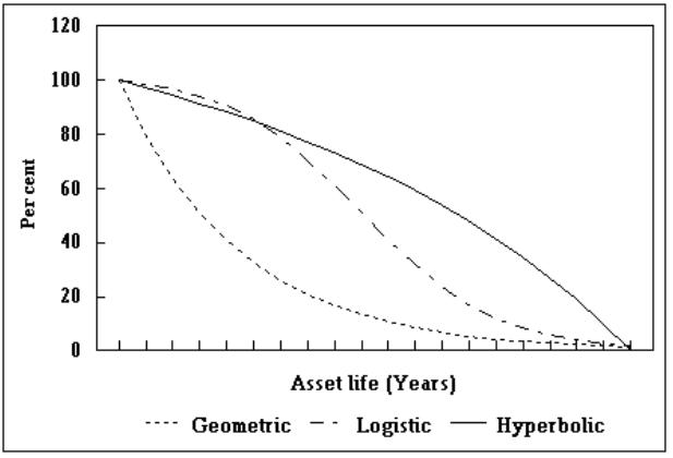
14.36 There is a lack of empirical data about the shape of age-efficiency functions and the choice is a matter of judgement. Although capital stock levels are sensitive to the shape of the age-efficiency function, average growth rates are not. (In fact, if real GFCF is held constant over time, the choice would have no impact on the capital stock growth rate, but it would affect the capital stock level.) The ABS has chosen to use hyperbolic functions, the same approach as that used by the US Bureau of Labor Statistics (BLS). In a hyperbolic function, the efficiency of the asset declines by small amounts at first and the rate of decline increases as the asset ages.
14.37 Hyperbolic decline has the form:
\(\large E_t = \frac{M-A_t }{M-bA_t }\)
where \(E_t\) is the efficiency of the asset at time \(t\) (as a ratio of the asset's efficiency when new).
\(M\) is the asset life as per the Winfrey distribution (discussed below)
\(A_t\) is the age of the asset at time \(t\)
\(b\) is the efficiency reduction parameter.
14.38 The efficiency reduction parameter b is set to 0.5 for machinery and equipment, and 0.75 for structures - the same parameter values as used by the US BLS. The higher value for non-dwelling construction redistributes efficiency decline to occur later in the asset's life, relative to machinery and equipment, the efficiency decline of which is distributed more evenly throughout the asset's life. For computer software, b is set to 0.5. For livestock, b is also set to 0.5. Clearly, a more accurate age-efficiency function and age-price function could be assumed by recognising that livestock are immature for a number of years before they begin service as mature animals. However, such improvements compromise model simplicity and the improvements from doing so would be quite small. For mineral exploration b is set to 1, implying that there is no efficiency decline in exploration knowledge. The opposite is the case for artistic originals, where b is set to 0, implying straight-line efficiency decline.
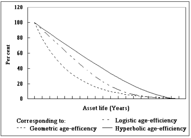
14.39 Graphs below show (i) the main types of age-efficiency functions and (ii) the age-price functions relating to each of the age-efficiency functions. When the hyperbolic functions for each of the possible lives of an asset are weighted together (as per the Winfrey distribution), the resulting average age-efficiency function resembles a logistic function with a point of inflection towards the end of its maximum life.
Graph 14.1 Age-efficiency functions
Graph 14.2 Age-price functions
Age-price functions
14.40 Age-price functions are calculated using average age-efficiency functions and a real discount rate. The age-efficiency function describes the decline in the flow of capital services of an asset as it ages. Using the discount rate, the net present value of future capital services can be readily calculated. For instance, when multiplied by a suitable scalar, the first value of the age-price function represents the present discounted value of the capital services provided by an asset over its entire life. The second value of the age-price function represents the present discounted value of the capital services provided by an asset from the end of its first year until the end of its life. The third value represents the present discounted value of the capital services provided by an asset from the end of its second year until the end of its life, and so on. Age-price functions are normalised and adjusted for mid-year purchase, to allow for some consumption of fixed capital occurring in the first year. The ABS has chosen a real discount rate of 4 per cent, the same as that used by the US BLS and which approximates the average real 10-year Australian bond rate.
14.41 When the net present values of the different assets are aggregated for a particular period, they form the net capital stock for that period.
Depreciation rate functions
14.42 In real terms, depreciation (or COFC) is the difference between the real economic value of the asset at the beginning of the period and at the end of the period. The depreciation rate function is calculated as the decline in the age-price function between assets of consecutive ages. When multiplied by a suitable scalar, it shows the pattern of real economic depreciation or COFC over an asset's life. Consumption of fixed capital for each vintage of each asset type is then aggregated to form the total consumption of fixed capital for that period. It can also be calculated as GFCF less the net increase in the net capital stock; that is, GFCF less the difference between the net capital stock at the end of the period and at the beginning of the period).
Sources and methods - Annual
The Perpetual Inventory Method (PIM)
14.43 The PIM measures capital stock and COFC annually. The steps involved in applying the PIM are summarised in the chart below.
Figure 14.1 The PIM process
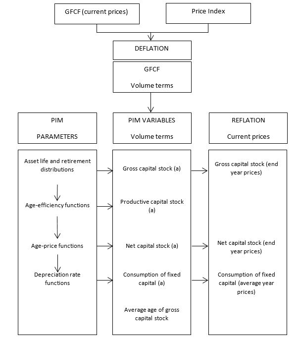
- Expressed in the average prices of the reference year
14.44 The PIM is applied to annual volume estimates of GFCF at a detailed level; that is, for a particular asset type for a particular industry in a particular institutional sector), in order to maintain an estimate of capital stock. It requires an initial estimate of capital stock, but this is taken to be zero. Volume estimates of net and productive capital stock and consumption of fixed capital are compiled using vector multiplication. The product of two vectors results in a value for a particular period. The first vector represents the age-efficiency or age-price or COFC pattern from when the fixed asset is new to the end of its life. The second vector is always the GFCF series. Shifting the second vector (GFCF) one year at a time before multiplying with the first vector results in a time series of values of capital stock or consumption of fixed capital, depending on the vector used.
14.45 For instance, gross capital stock at the end of period t is the product of the survival function and GFCF vectors. The first element of the GFCF vector is the value for period t; the second element is the value is for period t-1; the third is for period t-2; and so on. The final element is the value for period t-m, where m is the maximum possible life of the asset. A survival function represents the probability that a fixed asset is still in service and is derived from the asset life distribution. When the asset is new, the survival probability is equal to 1, but as it ages the survival probability declines, until it reaches zero. At the end of its life the asset is assumed to have a zero scrap value (in practice, it is recognised that positive and negative scrap values can occur but no attempt has been made to quantify the net effect of these). The survival function can be constructed by subtracting, for each period, the probability of retirement in that period.
14.46 Productive capital stock is the product of the average age-efficiency function (AAE) and GFCF vectors. The AAE for a particular asset age is calculated as a weighted average of the efficiency functions for each possible length of life, using the probability of retirement as weights.
14.47 Net capital stock is the product of the age-price function and GFCF vectors. Age-price functions are calculated using the AAE and a real discount rate in the following way. The present discounted value of the future stream of capital services from when the asset is new until the end of its life gives the first value of an age-price function, the present discounted value of the future stream of capital services from when the asset is one year old until the end of its life gives the second value, and so on. Age-price functions are normalised and adjusted on the assumption that all of GFCF in a year occurs mid-year.
14.48 COFC is the product of the depreciation rate function and GFCF vectors. The depreciation rate function is calculated as the decline in the age-price function between assets of consecutive ages.
14.49 Current price estimates at the most detailed level of estimation of gross capital stock, net capital stock and consumption of fixed capital are obtained by reflating the volume estimates. The price indexes used to reflate the volume estimates are the same as those initially employed to deflate GFCF except that, for capital stocks, they are adjusted to an end year basis by averaging consecutive values of the price indexes. For reflated consumption of fixed capital, which is a flow concept, the price indexes are not adjusted to an end of year basis. The resulting elemental series at current prices are aggregated to the level published, while elemental volume measures are aggregated to form chain volume measures at the level published. Elemental estimates of capital stock satisfy the following identities:
\(\large GKS_t = GKS_{t-1} + GFCF_t - R_t\)
\(\large NKS_t = NKS_{t-1} + GFCF_t - COFC_t\)
\(\large GKS$_t = (GKS_{t-1} + GFCF_t - Rt) * (PI_t + PI_{t+1}) / 2 \)
\(\large NKS$_t = (NKS_{t-1} + GFCF_t - COFC_t) * (PI_t + PI_{t+1}) / 2 \)
where
\(GKS_t=\) deflated gross capital stock in period \(t\)
\(NKS_t =\) deflated net capital stock in period \(t\)
\(GKS$_t =\) gross capital stock in current prices at end of period \(t\)
\(NKS$_t =\) net capital stock in current prices at end of period \(t\)
\(GFCF_t =\) deflated gross fixed capital formation in period \(t\)
\(R_t =\) deflated retirements in period \(t\)
\(COFC_t =\) deflated capital consumption in period \(t\)
\(PI_t =\) price index in period \(t\)
\($\) denotes the current dollar equivalent of the respective deflated series.
Note \(R_t\) is not included in the net estimates above as it is included in \(COFC\).
14.50 Average age of the gross capital stock at the end of each year is another output of the PIM. Average age is the age at 30 June of past years' GFCF weighted by their proportions of the surviving gross capital stock. These calculations assume an average mid-year purchase.
Current price GFCF
14.51 The GFCF data required as input into the PIM are consistent with those described previously, and are published in Australian System of National Accounts.
14.52 GFCF data by asset type are further classified by institutional sector and industry/purpose: dwellings; non-dwelling construction; machinery and equipment; cultivated biological resources; computer software; mineral and petroleum exploration; entertainment; literary or artistic originals; ownership transfer costs; research & development and weapons systems.
14.53 A number of problems with the generation of detailed capital formation estimates affect the reliability of estimates produced by the PIM. In particular, sector and industry estimates of private GFCF on machinery and equipment should be interpreted cautiously because the data available to adjust estimates in accordance with Australian Accounting Standard AASB16 and AASB117 (Accounting for Leases) are not as detailed as ideally required.
14.54 The first years for which estimates of capital stock and COFC have been published are 1966-67 and 1948-49, respectively. 1948-49 is the first year for which most national accounts data have been compiled by the ABS. Although the national accounts are compiled from 1959-60, in order to estimate capital stock and consumption of fixed capital from 1966-67 and 1959-60, respectively, estimates of GFCF are required for much earlier years. The length of the detailed GFCF series required varies depending on the particular mean asset life and asset life distribution applicable to that series.
14.55 Estimates of GFCF for years prior to 1948-49 are generally less accurate than those since 1948-49. The early data have relatively little impact on the present estimates because of the retirement of older assets, and the rapid growth of the Australian economy since World War II.
14.56 Estimates for years prior to 1948-49 are prepared using various sources including Butlin⁴⁶, and ABS data from issues of Production Bulletins, Primary Industry Bulletins, Secondary Industry Bulletins, Finance Bulletins, Transport and Communication Bulletins, State Statistical Registers and Australian and State Year Books.
14.57 Estimates of general government capital stock and consumption of fixed capital are calculated using the PIM by government purpose category. Estimates by purpose are then transformed into industries to obtain general government capital stock and consumption of fixed capital by industry. As the relationship between the government purpose classification and the ANZSIC is complex, this can only be done on an approximate basis.
Price indexes
14.58 The price indexes used in the PIM are the same as those used in the preparation of chain volume estimates of GFCF. However, the latter, with the exception of non-produced fixed asset estimates, are only compiled as chain volume estimates back to 1985-86. They are then linked to previously compiled constant price estimates at base years generally five years apart.
14.59 In contrast, the volume estimates derived as a means of estimating the capital stock related statistics are compiled all in one piece. The same is true for the reflation to derive current price estimates and chain volume estimates. This process requires the compilation of continuous price indexes going much further back in time than those required for the gross domestic product account.
14.60 For all categories other than construction, the price indexes extend no further back than 1948-49, but for construction they extend much further back. For years prior to 1948-49, the following price indexes are used:
- Dwellings and non-dwelling construction other than roads - a general building price index derived from Haig for the years 1938-39 to 1948-49.⁴⁷ For the years 1866 to 1938-39, a price index derived from Butlin.
- Roads - a roads price index derived from Keating, and Bureau of Transport Economics data (1941-42 to 1947-48).⁴⁸
14.61 As with the GFCF data, the poorer quality of early data should be considered in the light of its small contribution to more recent capital stock levels. Furthermore, unlike GFCF, most price indexes tend to be reasonably highly correlated over time.
14.62 The underlying price indexes from which the GFCF price indexes are compiled relate to a number of different base periods because of the length of the time series required. For example, ABS price indexes with base years of 1953-54, 1959-60, 1966-67, 1974-75, 1979-80, 1984-85 and 1989-90 are used, as well as non-ABS price indexes prior to 1948-49 which have earlier base years. Therefore, it is necessary to splice the price indexes with different base periods on the basis of relationships in overlapping periods.
14.63 Each item is a hybrid of several series, although only one price index series results for individual items. For example, price indexes for the early 1950s are used which reflect the composition of GFCF in 1953-54 when the current price values of machinery and equipment purchased in 1949-50 are calculated. In the mid to late 1950s, indexes which reflect the composition of GFCF in 1959-60 are used, etc.
Mean asset lives
14.64 The mean asset lives are the most important of the parameters used in the PIM. Together with asset life distributions, and the age-efficiency functions, they determine when assets are retired from the gross capital stock, the net capital stock, and the rate of depreciation charged. Six main data sources are used to derive estimates of mean asset lives:
- implicit tax lives;
- weighted prescribed tax lives;
- asset lives used by businesses to calculate depreciation for their own purposes;
- survival rates for vehicles in the motor vehicle fleet derived from data on new vehicle registrations and the motor vehicle census;
- technical information on the operating lives of various types of machinery from manufacturers' specifications; and
- asset life estimates from other OECD countries.
Changes in asset lives over time
14.65 Asset lives are influenced by a large number of variables, which may either increase or decrease asset lives over time. These variables include changes in rates of use, technological advances and quality changes.
14.66 In the case of motor vehicles there is strong evidence that mean lives have increased over the past fifty years, and these increases have been incorporated in the PIM for estimating the capital stock.
14.67 It is possible that the lives of other classes of assets have also changed, but there is no conclusive evidence to demonstrate that this has occurred.
14.68 While the lives of particular classes of assets may change over time, the average life span of all capital equipment also changes as a result of the changes in the composition of capital formation. This effect has been captured to some extent by breaking expenditure on machinery and equipment down into six major classes, as outlined below:
- Computers and peripherals equipment, encompassing laptops, tablets, PCs, printers and mainframes
- Electrical and electronic equipment, encompassing power generating equipment, transformers, batteries, solar panels and security equipment
- Motor vehicles encompassing cars, trucks, utes or any other vehicle where the primary use is to be driven on public roads
- Industrial machinery and equipment encompassing forklifts, conveyers, compressors, processing machinery or any other specialised equipment used for the operations of a business or organisation
- Other transport equipment, encompassing trailers, boats, ships, trains, aircraft or any other vehicle used in the transportation of people or goods
- Other equipment, encompassing equipment not elsewhere classified in the categories above.
14.69 Since the 1960s, there has been a steady increase in the use of computers, which in 1997-98 comprised about 12 per cent of capital formation on machinery and equipment. Computers are a relatively short-lived item of equipment and the increase in their use has had the effect of reducing average equipment lives.
14.70 The increased use of computers and the increased lives of motor vehicles have offsetting effects, with the net impact on equipment lives differing between industries according to the relative weights of computers and motor vehicles in their machinery and equipment expenditure. In industries where motor vehicles form a high proportion of machinery and equipment expenditure, such as agriculture, average lives have increased, while for industries such as finance and insurance, where computers form a relatively high proportion of capital formation, average equipment lives have fallen.
Machinery and equipment
14.71 Asset lives are estimated for the six classes of machinery and equipment. In calculating average asset lives, implicit tax lives (based on the inverse of the depreciation rates published in the 1997 Master Tax Guide) are used as a basic source of information. While implicit tax lives may change over time, they are regarded as being of insufficient accuracy to calculate changes in economic lives over time. They are, however, industry based and comprehensive in coverage. In principle they are based on industry information about the actual service lives of machinery and equipment. Nevertheless, information from other sources suggests that tax lives are, in general, shorter than economic lives, and additional sources have been used to estimate the actual economic lives of the various types of machinery and equipment.
14.72 The additional information sources are less comprehensive in coverage than the tax data, so selected items of machinery and equipment have been used to estimate ratios of tax lives to economic lives. The general approach has been to calculate a weighted average tax life for the various types of machinery and equipment employed in each industry, then supplementary sources, such as technical data and information collected from industry sources have been used to estimate the economic lives of assets employed in those industries. The estimates developed by Walters and Dippelsman have been adopted where no new information on economic lives has been available.⁴⁹ A ratio of economic lives to average tax lives has then been calculated. This ratio has been applied to all machinery and equipment employed in the industry to determine an average economic life.
14.73 The ratio of economic lives to tax lives differs between industries. For example, much of the machinery and equipment used in agriculture is similar to machinery and equipment used in mining and construction, and particular items of machinery and equipment, such as tractors, generally have the same prescribed tax life regardless of the industry in which they are employed. However, work practices differ between industries, with machinery and equipment engaged in agriculture generally being used less intensively than similar equipment in the construction or mining industries. Therefore, agricultural equipment can be expected to last longer than similar equipment engaged in construction or mining, and so the ratio of economic lives to tax lives is higher for agriculture than for construction or mining. In some cases, the lives of particular classes of machinery and equipment differ between industries; this is notably so in the case of electrical equipment. In the electricity, gas and water industry, electrical equipment is estimated to have an average life of 30.9 years, compared with an average life of 16.6 years for electrical equipment in other industries. This difference is due to an allowance being made for the longer life of the heavy electrical equipment used in the electricity, gas and water industry.
14.74 Asset lives for machinery and equipment in 1996-97 are reported in the table below for each industry. Due to a lack of information as to whether asset lives have been lengthening or shortening, the asset lives of all categories other than road vehicles and computers are held constant.
14.75 In the case of road vehicles, which constitute over 30 per cent of GFCF on machinery and equipment, average lives have been estimated using data on new vehicle registrations and the age composition of the vehicle fleet. Data are published in New Motor Vehicle Registrations, Australia: Preliminary and Motor Vehicle Census, Australia. For the census years, the number of vehicles of each vintage surviving in the stock has been related to the number of new registrations in the year of manufacture to calculate the percentage of survivals from the respective vintages. The results show a general decline over time as the older vehicles drop out of the stock. The point at which 50 per cent of vehicles manufactured in a particular year remain in the stock gives the median life of vehicles manufactured in that year. For example, if 50 per cent of the vehicles manufactured in 1960 (or more precisely first registered in 1960) remain in the stock in 1972, then this implies that the median life of vehicles manufactured in 1960 is 12 years. This technique has been used to estimate vehicle lives at the census dates, and lives for the intervening years have been calculated by interpolation. It is not possible to precisely calculate mean lives, as a proportion of vehicles have lives exceeding the range covered by the data available. However, analysis of the age distribution suggests that the median is a close approximation to the mean.
14.76 Vehicle lives are estimated using the above approach from 1950. Motor vehicle lives increased from 13.9 years to 18.7 years over the period, 1950 to 1979. It is not possible to measure the median lives of vehicles manufactured until half of them have actually lived out their lifespan and so for recent years this method is not applicable. For recent years a combination of data for the average age of the vehicle fleet and trends in the age profile of the fleet are used to project trends in vehicle lives. It is estimated that the mean life of motor vehicles manufactured in 1997 is 19.9 years.
14.77 The average life of computer equipment is assumed to have gradually declined from 8.5 years in 1960 to 5.4 years in 1997-98. This change is attributed to the decline in the proportion of mainframe computers relative to PCs and the longer lives of the former.
14.78 The table below outlines the mean asset lives (years) for machinery and equipment (excluding weapons systems) by type of equipment and industry.
| Industry | Computers & peripherals | Electrical & electronic equipment | Industrial machinery & equipment | Motor vehicles | Other transport equipment | Other plant & equipment |
|---|---|---|---|---|---|---|
| Agriculture, forestry & fishing | 5.4 | 16.5 | 21.7 | 19.9 | 16.5 | 17.8 |
| Mining | 5.4 | 17.8 | 19.9 | 19.9 | 17.8 | 16.5 |
| Manufacturing | 5.4 | 13.9 | 15.6 | 19.9 | 13.9 | 12.6 |
| Electricity, gas, water & waste services | 5.4 | 30.9 | 20.6 | 19.9 | 18.7 | 17.8 |
| Construction | 5.4 | 13.9 | 15.6 | 19.9 | 13.9 | 12.6 |
| Wholesale trade | 5.4 | 18.7 | 20.6 | 19.9 | 18.7 | 17.8 |
| Retail trade | 5.4 | 18.7 | 20.6 | 19.9 | 18.7 | 17.8 |
| Accommodation, & food services | 5.4 | 18.7 | 20.6 | 19.9 | 18.7 | 17.8 |
| Transport, postal & warehousing | 5.4 | 18.7 | 20.6 | 19.9 | 18.7 | 17.8 |
| Information media, & telecommunications | 5.4 | 15.6 | 17.8 | 19.9 | 15.6 | 14.9 |
| Finance and insurance services | 5.4 | 15.6 | 17.8 | 19.9 | 15.6 | 14.9 |
| Rental hiring & real estate services | 5.4 | 15.6 | 17.8 | 19.9 | 15.6 | 14.9 |
| Professional, scientific and technical services | 5.4 | 15.6 | 17.8 | 19.9 | 15.6 | 14.9 |
| Administration & support services | 5.4 | 15.6 | 17.8 | 19.9 | 15.6 | 14.9 |
| Public administration & safety | 5.4 | 15.6 | 17.8 | 19.9 | 15.6 | 14.9 |
| Education and training | 5.4 | 17.8 | 19.9 | 19.9 | 17.8 | 16.5 |
| Health care and social assistance | 5.4 | 15.6 | 17.8 | 19.9 | 15.6 | 14.9 |
| Arts and recreation services | 5.4 | 17.8 | 19.9 | 19.9 | 17.8 | 16.5 |
| Other services | 5.4 | 17.8 | 19.9 | 19.9 | 17.8 | 16.5 |
Weapons systems
14.79 The ABS has undertaken research on asset lives and retirement functions for each equipment type (aircraft, ships, ground equipment) using asset life information from the Australian Defence Force (ADF).
14.80 The ADF determines the current service life by subtracting the inception date from the planned withdrawal date for different weapon sub classes and this is seen as a suitable estimate of asset lives.
| Mean life (years) | ||
|---|---|---|
| Weapons systems | 27.8 | |
Non-dwelling construction
14.81 The estimated average lifespans of non-dwelling construction (including alterations and additions) are given in the table below. These estimates are based on the findings of Walters and Dippelsman.
14.82 These estimates have been checked against data on the age of buildings demolished in the Sydney and Melbourne central business districts over a ten-year period. The Sydney and Melbourne data broadly support the age estimates used by Walters and Dippelsman (1985), giving an average age at demolition of 62 years.
14.83 The short time span for which data are available and the relatively small number of buildings demolished over that period do not permit any significant conclusions to be drawn as to whether building lives have been increasing or decreasing over time. It can be argued, a priori, that as a result of economic and population growth the use of core infrastructure becomes more intensive (i.e. the flow of services from that infrastructure increases) and that, all things being equal, the life span of those facilities would be reduced. However, in the absence of clear empirical evidence to support that proposition, the asset lives used by Walters and Dippelsman have been retained.
Private corporations
14.84 Taxation lives are considered too short and lacking in discrimination between different industries and types of buildings. Unpublished data used in compiling the ABS publication, Building Activity, Australia were obtained showing separately new work and alterations and additions for different types of buildings. Alterations and additions are assumed to have an average asset life about half that of new work in that they can occur at most stages in the life of the primary building. Information on types of other construction for the private sector is obtained from the ABS publication, Engineering Construction Activity, Australia. Estimates are finalised on a subjective basis, taking into account lives used in other OECD countries, accounting estimates, and estimated proportions of new buildings, alterations and additions and non-building construction.
Public corporations
14.85 For public corporations, separate investigations are undertaken for electricity, gas and water; transport and storage; communication; accommodation, cafes and restaurants, cultural and recreational services; and personal and other services. Mean lives for public corporations are also reported separately in the table below. Together, these industries account for around 90 per cent of public corporations GFCF. For other industries, the estimates of private sector asset lives are used.
General government
14.86 Non-dwelling construction consists mostly of offices, schools, hospitals and roads. The average life of total non-dwelling construction is estimated to be 54 years, with new government buildings assumed to have the same average life as private commercial buildings of 65 years. As with private commercial buildings, the evidence as to whether the average lives of buildings are changing over time is inconclusive, and lives are assumed to remain constant over time. For non-dwelling construction on roads the mean asset lives used by Walters and Dippelsman (1985) have been retained.⁵⁰
Dwellings
14.87 The initial estimates used by Walters and Dippelsman have been retained up until 1985. However, recent analysis of demolitions data suggest that asset lives have declined in recent years due to obsolescence likely resulting from increasing land prices and demand for well-located land. The ABS has gradually reduced the asset lives of private brick dwellings from 88.1 years to 70 years and Alterations and additions from 39.5 years to 25 years to reflect changes in the economy over this time.
Ownership transfer costs
14.88 The treatment for ownership transfer costs in the PIM is unique. The cost of ownership transfer is written off over the period during which the acquirer expects to hold the asset. If the expectation is met, the costs of ownership transfers will be entirely depreciated when the asset is resold.
14.89 The table below outlines the mean asset lives (years) for non-dwelling construction, dwellings and ownership transfer costs by industry and institutional sector.
| Financial and non-financial corporations | Public non-financial corporations and general government | |||
|---|---|---|---|---|
| NON-DWELLING CONSTRUCTION | ||||
| Agriculture, forestry & fishing | 41.8 | 41.8 | ||
| Mining | 29.5 | 29.5 | ||
| Manufacturing | 38.6 | 38.6 | ||
| Electricity, gas, water & waste services | 55.3 | n.a. | ||
| Electricity and gas | n.a. | 37.9 | ||
| Water and waste services | n.a. | 71.6 | ||
| Construction | 44.5 | 44.5 | ||
| Wholesale trade | 50.6 | 38.6 | ||
| Retail trade | 50.6 | 38.6 | ||
| Transport, postal & warehousing | 40.6 | n.a. | ||
| Urban transport | n.a. | 51.9 | ||
| Road and rail transport | n.a. | 67.0 | ||
| Sea transport | n.a. | 47.5 | ||
| Air transport | n.a. | 30.9 | ||
| Other transport, postal & storage services | n.a. | 49.1 | ||
| Information, media, & telecommunications | 40.6 | 49.1 | ||
| Accommodation & food services | 50.6 | 41.7 | ||
| Financial & insurance services | 57.3 | n.a. | ||
| Rental hiring & real estate services | 57.3 | 57.3 | ||
| Professional, scientific and technical services | 57.3 | 57.3 | ||
| Administration & support services | 57.3 | 57.3 | ||
| Public administration & safety | n.a. | 54.1 | ||
| Education & training | 50.6 | 50.6 | ||
| Health care and social assistance services | 50.6 | 50.6 | ||
| Arts and recreation services | 50.6 | 50.6 | ||
| Other services | 50.6 | 50.6 | ||
| General government (all industries except Defence and roads) | n.a. | 54.1 | ||
| Defence | n.a. | 38.6 | ||
| Roads | n.a. | 33.4 | ||
| DWELLINGS | ||||
| Private brick homes | 70.0 | n.a. | ||
| Private timber, fibro and other houses | 58.9 | n.a. | ||
| Private non-house dwellings (units, flats, etc.) | 58.9 | n.a. | ||
| Private alterations and additions | 25.0 | n.a. | ||
| Public | n.a. | 58.9 | ||
| OWNERSHIP TRANSFER COSTS | ||||
| Dwellings | 17.0 | n.a. | ||
| Non-dwelling construction | 30.9 | n.a. | ||
Cultivated biological resources
Livestock
14.90 Information about mean asset lives of breeding and dairy cattle, and wool producing sheep, were obtained from several industry bodies; namely, Bureau of Rural Sciences; Woolmark Company; Dairy Farmers Corporation; and Meat and Livestock Association. Asset lives used are: breeding cattle stock – mean seven years; dairy cattle – mean ten years; and sheep for wool – mean six years. The same method is used for thoroughbred horses, standardbred horses, other horses and pigs for breeding, due to the limited information available to calculate the asset lives of these biological resources.
Orchard growth
14.91 There are three components of capital estimates, namely, orchard fruit and nut trees, plantation fruit bearing plants, and grapevines. These have different asset lives due to the types of plants.
14.92 The table below outlines the mean asset lives (years) for cultivated biological resources.
| Mean life (years) | |
|---|---|
| Livestock | |
| Sheep (wool) | 6.4 |
| Dairy | 10.3 |
| Breeding cattle | 7.5 |
| Thoroughbred horses | 10.3 |
| Standardbred horses | 10.3 |
| Other horses | 10.3 |
| Pigs for breeding | 8.5 |
| Orchards | 29.5 |
| Plantations | 7.5 |
| Grapevines | 40.6 |
Intellectual property products
Research & development
14.93 The value of R&D capital depreciates over time as new innovations emerge. As this occurs, earlier R&D becomes less effective in the production process and contributes less to profitability. Because of the intangible nature of the asset, the decline in value is difficult to measure and most studies use a range of assumptions based on econometric studies or the observed retirement rates for patents. The Australian Industry Commission report on Research and Development (1995) cites work by Mansfield (1973) and Pakes and Shankerman (1978, 1984), suggesting that industrial knowledge depreciates faster than physical capital with little left after 10 years. More recent studies have suggested that the rate of technological change, and consequently the rate of obsolescence, has increased in recent years (Caballero and Jaffe, 1993). Data on patent expiry rates suggest considerably longer asset lives.
14.94 Data compiled by Intellectual Property Australia show that the mean lifespans of standard patents filed in Australia between 1980 and 2001 were between 10 and 13 years. The data are categorised by 'technology group', whereas R&D expenditure data are categorised by industry (to sub-division level). There is no simple correspondence between the technology group classification and the industry classification; however, there are relatively small differences between the mean patent lives for different technology groups. Given the difficulties in producing estimates for individual industries, and the fact that the estimates (based on the patent data) do not differ greatly, a single asset life distribution is used for all R&D in the ASNA. A mean asset life of 11.3 years has been derived from a weighted average of the patent lives of the different technology groups.
14.95 Patent lives do not necessarily represent the lives of all R&D products and, in principle, an adjustment should be made to account for the fact that not all R&D is patented. Although it seems reasonable to expect that non-patented R&D would on average have shorter lives and depreciate faster than patented R&D, empirical estimates based on econometric studies vary greatly (with some of the evidence suggesting a longer life than that estimated from patents). In the United States in 2007, the Bureau of Economic Analysis (BEA) tested four scenarios, with the first scenario based on a 15 per cent annual depreciation rate. The other scenarios were based on more rapid rates of technological change, and consequently more rapid rates of obsolescence. The assumption of shorter economic lives gives greater weight to more recent innovations in the capital stock estimates.
14.96 A mean asset life of 11.3 years is broadly consistent with international results. A recent draft OECD Handbook states that the different approaches to estimating R&D asset lives 'generally indicate that service lives lie between 10 and 20 years'.⁵¹ However, most countries have not committed to an estimate and/or method to be used in their national accounts (the US figures have been used in the BEA's R&D Satellite Account). None of the OECD countries use an asset life significantly shorter than 10 years. For many countries only a depreciation rate is specified, but under a standard double declining balance assumption (that is double that of a straight-line depreciation) they imply similar (or sometimes longer) lives. Given the lack of evidence to the contrary, the ABS has assumed a mean asset life of 11.3 years based on patents data.
Computer software
14.97 It is important to distinguish between the different types of software because they are known to have different asset lives, partly due to the different lives of mainframe and personal computers. The software 'mix' has also been changing over time, in favour of PC-based software.
- In-house and customised software – information has been obtained from academic papers and Gartner research, although empirical evidence is quite weak. For years up to 1988-89, a mean life of eight years has been chosen. From 1989-90, the greater incidence of outsourcing software development, combined with increased technological change, is believed to result in shorter lives, and so a mean life of 6.5 years has been used.
- Purchased (packaged) software – for years up to 1988-89, a mean life of six years has been chosen. From 1989-90, average and maximum lives fall by about 2 years to reflect the impact of greater technological change; thus, average lives fall from 6 to 4.5 years in 1989-90.
Entertainment, literary or artistic originals
14.98 Music – general information about the life cycle of typical Australian music titles is obtained from the Australian Record Industry Association (ARIA). Indications point to an average life of about 3 years. However, detailed information is not obtained from ARIA's membership to verify the accuracy of these indications.
14.99 Film and TV – it is difficult to attribute an asset life to film as little is known about the percentage of films that continue to generate revenue for periods greater than one year, two years etc. However, information from the Australian Film Commission, and from Martin Dale's book The Movie Game - the film business in Britain, Europe and America, indicated that an average life of 3.5 years would be appropriate.
14.100 Literary – information is obtained from the Australian Publishers Association's (APA) booklet, Introduction to Book Publishing, and from enquiries to large publishers. APA recognises that books have a very short life. An average life of 2.7 years was proposed, and there were no objections to this estimate in discussions with experts from the APA and other large publishers. However, the increasing availability of new print technology such as 'print on demand' could redistribute the author's income, and therefore the life of book titles, over a longer period in the future.
Mineral exploration
14.101 Asset lives for mineral exploration are assumed to coincide with mine and oilfield lives. These are derived indirectly using economic demonstrated resources (EDR) from the balance sheets. First, average annual production for each commodity is divided into its EDR to derive the asset life for each commodity. Using exploration expenditure proportions for each commodity as weights, the average lives for the commodities are aggregated to an average mine life for all commodities. The average mine life used for mineral exploration is 34.5 years.
14.102 Mine lives for some commodities, namely black coal, iron ore and uranium, have extremely long asset lives, and are excluded from the calculation to avoid distorting the average life. These items had a much greater proportion of total exploration expenditure in early years, but their inclusion would lead to an unjustifiably strong decline in the overall average life of mineral exploration over time.
14.103 The table below outlines the mean asset lives (years) for intellectual property products.
| Mean life (years) | ||
|---|---|---|
| Computer software | ||
| In-house & customised (a) | 6.5 | |
| Purchased (b) | 4.5 | |
| Artistic originals | ||
| Film & TV | 3.5 | |
| Music | 2.7 | |
| Literary | 2.7 | |
| Exploration | 34.5 | |
| Research & Development | 11.3 | |
a. Prior to 1989-90, the mean life is 8 years
b. Prior to 1989-90, the mean life is 6 years
Asset life distributions
14.104 The PIM is applied at a relatively high level of disaggregation, with each component of GFCF consisting of a large variety of individual assets, each with its own life span. Even within particular types of assets, variations in lives will occur because of differences in the rate of use, maintenance etc. Because of the lack of recent empirical evidence, asset life distribution curves developed by Winfrey in 1938 are used.⁵² The Winfrey S3 is a bell-shaped symmetric curve, with approximately three quarters of assets retiring within 30 per cent of the mean asset life. It is empirically based, related to variations in lives of particular types of assets, and is consistent with the general presumption that the expected life for a particular asset will follow an approximately normal distribution.
Endnotes
Sources and methods - Quarterly
14.105 The PIM measures COFC annually due to its parameters. Linear interpolation and extrapolation are used to estimate quarterly COFC.
| Item | Comment |
|---|---|
| Consumption of fixed capital | The Perpetual Inventory Method measures consumption of fixed capital annually due to its parameters. Linear interpolation and extrapolation are used to estimate quarterly consumption of fixed capital. |