APPENDIX 3 GINI COEFFICIENT AND OTHER SINGLE STATISTIC SUMMARIES OF INCOME DISTRIBUTION
INTRODUCTION
Taken together, the simple measures of income distribution such as mean, median, percentile ratios and income shares (described in Section 1.6 'Gini coefficient and other measures of income distribution') can provide an indication of changes in the income distribution of a population over time, or differences in the income distributions of two separate populations. However, none of the simple measures comprises a single statistic that summarises the whole income distribution in a way that directly takes into account the individual incomes of all members of the population. This appendix considers some of the issues associated with compiling a single statistic summary of inequality, and compares a number of alternative measures. The first is the Gini coefficient, which is the most commonly used summary measure. The Gini coefficient is compared with the Theil index and a number of Atkinson indexes.
Note that the analysis in this appendix has been carried out using data from the 2002-03 and earlier SIHs.
CONCEPT OF INCOME INEQUALITY
It is generally agreed that perfect equality in the distribution of income can be defined as the situation in which everyone in the population lives in a household with the same equivalised disposable household income (see Section 1.3 'Equivalised household income'). If any person has lower or higher equivalised disposable household income than any other person, there is inequality in the income distribution.
However, there is no unique, generally accepted way of summarising the degree to which a population does not have perfect equality, or, more practically, summarising the difference in inequality between two populations. Unequal distributions of income can occur in many different ways. The majority of people may have very similar incomes with pockets of very high or very low income. Or entire populations may be heavily clustered at the top and the bottom of the income distribution with few people receiving incomes in between these extremes. To evaluate one income distribution as having greater or lesser inequality than another income distribution, it is necessary to compare the distributions in terms of which segments of the population have a greater share of income and which segments have a lower share. It is then necessary to at least implicitly judge whether the relative gain in income by some people is more than offset or less than offset by the relative loss of income by some other people. Different observers may make different judgments about the same situation, depending on personal preferences, etc. Different summary measures of inequality embody different judgments about the relative gains and losses. As will be seen below, some measures allow the user to explicitly set a parameter to reflect the judgment of the user in this regard.
Simple examples of different patterns of inequality can be used to illustrate the issues under consideration.
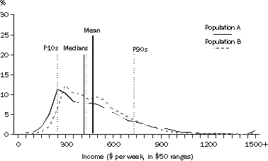
For the first example, consider the equivalised disposable household income of the two populations A and B depicted in the graph A3.1, 'Frequency Distributions I'. Population A is derived from the 2000-01 SIH population after removing people in households with zero income (the reason for deleting households with zero income is explained later in this appendix). Population B covers the same people as in population A, but everyone's income is transformed in a particular way that reduces the proportional differences in income across the population while retaining the same mean income for the population. There are therefore fewer people on very low or very high incomes and more people in between these extremes, with the median for population B closer to the mean, and less spread between P10 and P90.
A3.1 FREQUENCY DISTRIBUTIONS I
The extent to which the income distributions for populations A and B vary from equality, and from each other, can be illustrated graphically another way, using Lorenz curves.
LORENZ CURVES
The Lorenz curve is a graph with the horizontal axis showing the cumulative proportion of the persons in the population ranked according to their income and with the vertical axis showing the corresponding cumulative proportion of equivalised disposable household income. The graph then shows the income share of any selected cumulative proportion of the population. The diagonal line represents a situation of perfect equality, that is, all people have the same equivalised disposable household income. The graph A3.2, 'Lorenz Curves I' shows the Lorenz curves for the two populations described above.
A3.2 LORENZ CURVES I
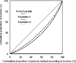
Since the distribution of population B's income is uniformly less widely spread than for population A, all points of the Lorenz curve for population B are closer to the line of perfect equality than the corresponding points of the Lorenz curve for population A. In this situation, population B is said to be in a position of Lorenz dominance and can be regarded as having a more equal income distribution than population A.
However, if the Lorenz curves of two populations cross over there is no Lorenz dominance and there is no generally accepted way of defining which of the two populations has the more equal income distribution.
Consider the income distributions of the populations in a second example, as shown in the graph A3.3 'Frequency Distributions II'. Population A is the same as in the first example above. Populations C and D also cover the same people as in population A, and all have the same mean income. But the income of populations C and D are transformed in such a way that the lower income people are relatively better off than for population A and the higher income people are also relatively better off than for population A. Conversely, the incomes of the middle of the population are relatively reduced so that the mean income of the three populations remains the same. Also the ranking of the population by income has not changed the relative position of any person. For population A, the lowest income is $1, for population C it is about $180, and for population D it is about $150. The incomes of the higher income people have received a relatively greater boost for population D than for population C.
A3.3 FREQUENCY DISTRIBUTIONS II
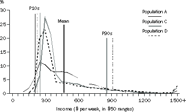
The medians (not shown in the graph) are higher for populations C and D than for A, but all are below the mean. As for population B in the earlier graph, P10 for populations C and D is above P10 for population A. However, in contrast to population B, populations C and D also have P90 above that of population A.
The graph A3.4, 'Lorenz Curves II' shows the resultant differences in the Lorenz curves, with the curves for both populations C and D crossing that of population A. Therefore there is ambiguity about whether populations C and D have greater or less income inequality than population A. Comparing populations C and D to population A, both lower and higher income people have a greater share of total income and middle income people have less. In population C, the lower income people show a relatively greater gain than the higher income people. Conversely, in population D, the higher income people show a relatively greater gain than the lower income people. However, the curve for population C does not cross that of population D, and therefore population C has Lorenz dominance over population D, that is, income is unambiguously distributed more equally in population C than in population D.
A3.4 LORENZ CURVES II
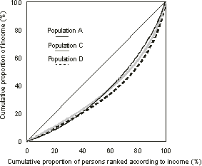
Table A3.5 shows the years for which the income distribution has Lorenz dominance over the income distributions of other years. Table A3.5 also shows the years for which the lack of Lorenz dominance is due only to the crossing of the Lorenz curves in the bottom decile of the income distribution, that part of the income distribution for which income is not necessarily a good indicator of economic wellbeing.
The Lorenz curves described in this appendix are depicting the relativities between income distributions and do not show whether incomes overall have been growing, contracting or remaining static. Another form of Lorenz curves, known as Generalised Lorenz curves, depict the cumulative incomes of populations after adjusting for differences in average income between the populations. They therefore can be used to analyse differences in the level of income as well as differences in distribution, but do not as clearly show differences in inequality (see, for example, Deaton (1997)).
SUMMARY INDICATORS
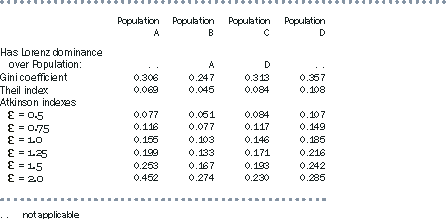
The three commonly used summary inequality measures mentioned earlier - the Gini coefficient, the Theil index, and the Atkinson index - can be produced for populations A, B, C and D. Table A3.6 provides the values for these measures with respect to each population, and descriptions of the measures follow. The Atkinson index is considered with a number of different settings of a user defined parameter, as described later.
A3.6 COMPARISON OF INEQUALITY SUMMARY STATISTICS
GINI COEFFICIENT
The Gini coefficient can be defined by referring to the Lorenz curve. It is the ratio of the area between the actual Lorenz curve and the diagonal (or line of equality) compared to the total area under the diagonal. The Gini coefficient equals zero when all people have the same level of income and approaches one when one person receives all the income. In other words, the smaller the Gini coefficient the more equal the distribution of income, given the assumptions underlying the Gini coefficient.
Table A3.6 shows that the Gini coefficient for population B is substantially below the coefficient for population A. The coefficient for population C is a little above that for population A, and the coefficient for population D is somewhat further above. According to the Gini coefficient, therefore, population B has a more equal income distribution than population A, but populations C and D have less equal distributions.
Mathematically, the Gini coefficient can be expressed as
where
n is the number of people in the population
 is the mean equivalised disposable household income of all people in the population
and yi and yj are the equivalised disposable household income of the ith and jth persons in the population.
The Gini coefficient is a summary of the differences between each person in the population and every other person in the population. The differences are the absolute arithmetic differences, and therefore a difference of $x between two relatively high income people contributes as much to the index as a difference of $x between two relatively low income people.
An increase in the income of a person with income greater than median income will always lead to an increase in the coefficient, and a decrease in the income of a person with income lower than median income will also always lead to an increase in the coefficient. The extent of the increase will depend on the proportion of people that have income in the range between median income and the income of the person with the changed income, both before and after the change in income. At the extremes, increasing the income of the person with the lowest income by $x or increasing the income of the person with the highest income by $x will respectively decrease and increase the Gini coefficient by the same amount (assuming the lowest income person remains the lowest income person after the change).
THEIL INDEX
Another commonly used summary statistic is the Theil index, which can be expressed mathematically as
The Theil index ranges between zero when all incomes are equal and log n when one person receives all the income. It therefore has a higher value if one person in a larger population receives all income compared to if one person in a smaller population receives all income. However, it has the same value for two unequally sized populations if income is distributed with the same proportions in the two populations, that is, they have identical Lorenz curves. (The other single statistic summary indicators discussed in this appendix also have this characteristic.)
As for the Gini coefficient, if one population has Lorenz dominance over another population, the Theil index for the first population will be lower. Table A3.6 shows, therefore, that population B has a lower Theil index than population A, and population C has a lower Theil index than population D. The Theil index for population A is also below that for populations C and D.
The construction of the Theil index is substantially different from that of the Gini coefficient. Instead of comparing the income of each person with the income of every other person, the Theil index compares the income of each person with the mean income of the population.
ATKINSON INDEX
The Atkinson index is a more complex summary statistic. As in the Theil index, it contains a ratio comparison of each person's income with the population mean. But it also requires the user to set a parameter,  , specifying a level of 'inequality aversion'. The mathematical expression is
for

not equal to one, and
for

equal to one.
An Atkinson index always has a value between zero and one, regardless of the value of  . For any given value of
  , a lower value of the Atkinson index implies a greater degree of equality in the income distribution.
The 'inequality aversion' parameter,  , in effect specifies how much more benefit the user thinks an extra dollar would provide to a person with lower income compared to the benefit an extra dollar would provide to a person on a higher income. At the extreme of
  set to zero, the user has no 'inequality aversion'. The benefit of an extra dollar is assumed to be the same for everyone in the population, and the Atkinson index is always equal to zero regardless of whether the incomes in the population are widely dispersed or not.
The higher the setting of  , the greater the relative benefit derived by a lower income person receiving an extra dollar compared to a higher income person receiving an extra dollar. Consequently, the higher the setting of
  , the more sensitive is the Atkinson index to the ratios of the lowest incomes in the population to the mean income of the population. In particular, if a population has a number of people with income very close to zero, that is, only a very small proportion of mean income, their influence can dominate the Atkinson index and it has a value close to one.
Table A3.6 presents the Atkinson index with various settings of  between 0.5 and 2.0. As expected, the Atkinson indexes for population B are always lower than those for population A, reflecting the Lorenz dominance of population B over population A. Similarly, the Atkinson indexes for population C are always lower than those for population D. However, comparing populations C and D with populations A and B gives a mixed picture.
The higher the setting of  , the more emphasis the Atkinson index gives to the lowest values in the income distribution. Populations A and B have some values less than one hundredth of the mean, but populations C and D do not. Therefore the Atkinson index increases more quickly for populations A and B as the setting of
  is increased. For
  set to 1.0 and above, population A is measured as having greater income inequality than population C; for
  set to 1.5 and above population A has greater income inequality than population D; and for
  set to 2.0 population B also has greater income inequality than population C.
A complicating factor is that the Atkinson index cannot be calculated for a population containing zero incomes. Over one per cent of the SIH population has zero equivalised disposable household income including reported negative incomes which are set to zero when equivalised.
COMPARISON OF SUMMARY MEASURES
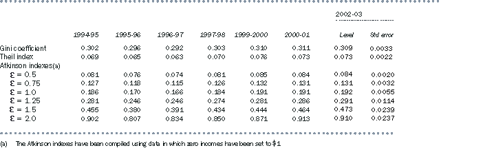
Table A3.7 provides the chosen summary measures for all years in which the SIH has been conducted up to 2002-03, together with the standard errors of the estimates in 2002-03. In 1995-96, 1997-98 and 1999-2000 all indicators consistently pointed to an increase or a decrease in inequality. In the other years there was a mixed picture. Over the whole period, all indicators show an increase in inequality, although none of the movements are significant at the 95% confidence level. Standard errors for years prior to 2002-03 tend to be higher than those for 2002-03 because the 2002-03 SIH had a larger sample than the earlier SIHs.
A3.7 SUMMARY STATISTICS OF INCOME INEQUALITY, 1994-95 TO 2002-03
SENSITIVITY OF SUMMARY MEASURES TO LOW INCOMES
Table A3.8 compares the impact on selected inequality summary statistics for the 2000-01 SIH population if persons with zero equivalised disposable household income have their income set to 1 cent, to 10 cents or to $1, or if they are omitted from the population altogether. Note that population A used in the first part of this appendix was the 2000-01 SIH population, after removing persons with zero income.
The table shows that the Atkinson indexes, but not the Gini or Theil measures, are sensitive to small changes, in dollar terms, to the lowest incomes in the Australian data set. It also shows that if persons with zero income are omitted from the population altogether, all indicators are impacted, with the least impact being on the Gini coefficient, and with an impact of over 50% on the Atkinson index with  set to 2.0.
A3.8 COMPARISON OF ALTERNATIVE TREATMENTS OF PERSONS WITH ZERO HOUSEHOLD INCOME, 2000-01
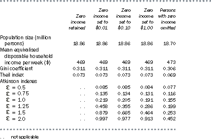
Given the likelihood that most of the very low incomes do not accurately represent the economic wellbeing of the respondents reporting such values, there is some doubt about the usefulness of summary indicators that are particularly sensitive to this segment of the population.
CHOICE OF SUMMARY MEASURES
There are several implicit and explicit assumptions underlying the measures discussed above. The Atkinson index explicitly requires the user to choose an 'inequality aversion' factor, but the other measures also implicitly embody judgements about how inequality is to be quantified.
Rather than considering just one summary measure, analysts will often look at a range of measures to see whether or not they give a consistent indication about changes in inequality, especially if there is no Lorenz dominance among the distributions being compared. Comparisons can be for the same population over time, or between different populations at a point in time.
Each of the indicators has its own particular advantages. For example, the Gini coefficient can be easily understood through the graphical interpretation of the Lorenz curve, and it is probably the most widely used indicator. The Theil index is particularly useful where analysts wish to decompose the measure of income inequality in a population into the inequality that exists within subpopulations and the inequality that exists between those subpopulations. The Atkinson indexes highlight that summary measures depend on the underlying assumptions about the quantification of inequality and assist the user in varying some of those assumptions. The Gini coefficient is sometimes criticised as being too sensitive to relative changes around the middle of the income distribution. This sensitivity arises because the derivation of the Gini coefficient reflects the ranking of the population, and ranking is most likely to change at the densest part of the income distribution, which is likely to be around the middle of the distribution.
In choosing which income distribution indicators to present, whether for simple or summary measures, it is useful to recall that income alone is not a perfect measure of the economic resources available to people to maintain or enhance their wellbeing, but it is a reasonable proxy that will be suitable for most people. However, as explained in section 1.5 'Low income households', some respondents report extremely low and even negative incomes in the Survey of Income and Housing (SIH), often reflecting their business and investment arrangements rather than any distinctly low economic wellbeing of these respondents. In other cases, incomes may be underreported either accidentally or deliberately, so again they are not a good indicator of economic inequality. It has therefore been considered inappropriate for these records to have a disproportionate influence on a summary income inequality measure being used for assessing inequality in economic wellbeing, just as the bottom decile is excluded in ABS publications from analysis of low income growth over time.
The Gini coefficient is the only single statistic summary of income distribution included in the published output from the SIH because it is not overly sensitive to the extremely low incomes that can be reported, and it is relatively simple to interpret. The other summary measures looked at in this appendix are more sensitive in the Australian context to extremely low and negative incomes that are assumed to not adequately reflect economic wellbeing.
Deaton, A. (1997). The analysis of household surveys: A microeconomic approach to development policy. John Hopkins University Press and The World Bank.
 Print Page
 Print All