TECHNICAL NOTE
DATA QUALITY
RELIABILITY OF THE ESTIMATES
1 Since the estimates in this publication are based on information obtained from a sample, they are subject to sampling variability. That is, they may differ from those estimates that would have been produced if all dwellings had been included in the survey. One measure of the likely difference is given by the standard error (SE), which indicates the extent to which an estimate might have varied by chance because only a sample of dwellings (or households) was included. There are about two chances in three (67%) that a sample estimate will differ by less than one SE from the number that would have been obtained if all dwellings had been included, and about 19 chances in 20 (95%) that the difference will be less than two SEs.
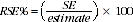
2 Another measure of the likely difference is the relative standard error (RSE), which is obtained by expressing the SE as a percentage of the estimate:
3 RSEs for count estimates from the 2013-14 Patient Experience Survey (using combined data from the MPHS and the HSS) have been calculated using the Jackknife method of variance estimation. This involves the calculation of 30 'replicate' estimates based on 30 different subsamples of the obtained sample. The variability of estimates obtained from these subsamples is used to estimate the sample variability surrounding the count estimate.
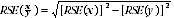
4 Proportions formed from the ratio of two estimates are also subject to sampling errors. The size of the error depends on the accuracy of both the numerator and denominator. A formula to approximate the RSE of a proportion has been used:
5 Data Cubes (spreadsheets) containing all tables produced for this publication and the calculated RSEs for each estimate are available from the Downloads tab of the publication. For illustrative purposes the RSEs for an excerpt of Table 5 have been included at the end of this Technical Note.
6 Only estimates (numbers and proportions) with RSEs less than 25% are considered sufficiently reliable for most purposes. Estimates with RSEs between 25% and 50% have been included and are annotated to indicate they are subject to high sample variability and should be used with caution. In addition, estimates with RSEs greater than 50% have also been included and annotated to indicate they are considered too unreliable for general use. All cells in the Data Cube with RSEs greater than 25% contain a comment indicating the size of the RSE. These cells can be identified by a red indicator in the corner of the cell. The comment appears when the mouse pointer hovers over the cell.
CALCULATION OF STANDARD ERROR
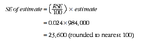
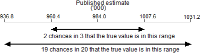
7 SEs can be calculated using the estimates (counts or proportions) and the corresponding RSEs. For example, Table 5.1 shows that the estimated number of males in the 15 to 24 (years) age group who needed to see a GP was 984,000. The RSE table corresponding to the estimates in Table 5.1 shows the RSE for this estimate is 2.4% (the 'Relative Standard Errors' section at the end of this Technical Note provides an excerpt of Tables 5.1 and 5.2). The SE is calculated by:
8 Therefore, there are about two chances in three that the actual number of males in the 15 to 24 age group who needed to see a GP was in the range of 960,400 to 1,007,600 and about 19 chances in 20 that the value was in the range 936,800 to 1,031,200. This example is illustrated in the diagram below.
PROPORTION AND PERCENTAGES
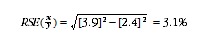
9 Proportions and percentages formed from the ratio of two estimates are also subject to sampling error. The size of the error depends on the accuracy of both the numerator and the denominator. A formula to approximate the RSE of a proportion is given below. The formula is only valid when the numerator is a subset of the denominator:

10 As an example, using estimates from Table 5.1, of the 984,000 males in the 15 to 24 age group who needed to see a GP, 59.7%, that is 587,900 males have a preferred GP. The RSE for 587,900 is 3.9% and the RSE for 984,000 is 2.4% (the 'Relative Standard Errors' section at the end of this Technical Note provides an excerpt of Tables 5.1 and 5.2). Applying the above formula, the approximate RSE for the proportion of males in the 15 to 24 age group who needed to see a GP who had a preferred GP is:
DIFFERENCES
11 Published estimates may also be used to calculate the difference between two survey estimates (numbers or proportions). Such an estimate is also subject to sampling error. The sampling error of the difference between two estimates depends on their SEs and the relationship (correlation) between them. An approximate SE of the difference between two estimates (x-y) may be calculated by the following formula:
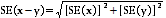
12 While this formula will only be exact for differences between separate and uncorrelated characteristics or sub populations, it provides a good approximation for the differences likely to be of interest in this publication.
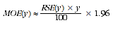
13 Another measure (which is not presented in this publication) is the Margin of Error (MOE), which describes the distance from the population value of the estimate at a given confidence level, and is specified at a given level of confidence. Confidence levels typically used are 90%, 95% and 99%. For example, at the 95% confidence level the MOE indicates that there are about 19 chances in 20 that the estimate will differ by less than the specified MOE from the population value (the figure obtained if all dwellings had been enumerated). The 95% MOE is calculated as 1.96 multiplied by the SE.
14 The 95% MOE can also be calculated from the RSE by:
15 MOEs at the 95% confidence level can easily be converted to a 90% confidence level by multiplying the MOE by

or to a 99% confidence level by multiplying by a factor of

16 A confidence interval expresses the sampling error as a range in which the population value is expected to lie at a given level of confidence. The confidence interval can easily be constructed from the MOE of the same level of confidence by taking the estimate plus or minus the MOE of the estimate.
SIGNIFICANCE TESTING
17 A statistical significance test for any comparisons between estimates can be performed to determine whether it is likely that there is a difference between two corresponding population characteristics. The standard error of the difference between two corresponding estimates (x and y) can be calculated using the formula in paragraph 11. The standard error is then used to create the following test statistic:

18 If the value of this test statistic is greater than 1.96 then there is evidence, with 95% confidence, of a statistically significant difference in the two populations with respect to that characteristic. Otherwise, it cannot be stated with confidence that there is a real difference between the populations with respect to that characteristic.
RELATIVE STANDARD ERRORS
19 The estimates and RSEs for an excerpt of Tables 5.1 and 5.2 are included below:
Table 5 Persons 15 years and over, Experience of GP services in the last 12 months by age and sex |
|
 | | Age group (years) |
| | 15 - 24 | 25 - 34 | 35 - 44 | 45 - 54 | 55 - 64 | 65 - 74 | 75 - 84 | 85 and over | Total |
ESTIMATE ('000)
|
| Males | | | | | | | | | |
| Has preferred GP | 587.9 | 666.6 | 796.5 | 900.3 | 953.9 | 777.8 | 434.1 | 95.1 | 5 210.1 |
| Total needed to see a GP | 984.0 | 1 133.6 | 1 154.4 | 1 146.8 | 1 101.8 | 853.6 | 460.1 | 100.3 | 6 936.8 |
PROPORTION (%)
|
| Males |
| Has preferred GP | 59.7 | 58.8 | 69.0 | 78.5 | 86.6 | 91.1 | 94.4 | 94.7 | 75.1 |
| Total needed to see a GP | 100.0 | 100.0 | 100.0 | 100.0 | 100.0 | 100.0 | 100.0 | 100.0 | 100.0 |
RSE OF ESTIMATE (%)
|
| Males | | | | | | | | | |
| Has preferred GP | 3.9 | 2.2 | 2.0 | 1.5 | 1.5 | 0.8 | 2.4 | 8.1 | 0.7 |
| Total needed to see a GP | 2.4 | 1.8 | 1.1 | 1.1 | 1.0 | 0.8 | 2.0 | 8.8 | 0.5 |
RSE OF PROPORTION (%)
|
| Males |
| Has preferred GP | 3.1 | 1.2 | 1.7 | 1.0 | 1.0 | 0.2 | 1.4 | 8.1 | 0.5 |
| Total needed to see a GP | - | - | - | - | - | - | - | - | - |
 Quality Declaration
  Print Page
 Print All