- About this Release
- A Guide to Interpreting Time Series - Monitoring Trends: An Overview, Jan 1995 (Feature Article)
- Employees and their Working Arrangements, Mar 1995 (Feature Article)
- Renters in Australia, Apr 1995 (Feature Article)
- Training Australia's Workers, May 1995 (Feature Article)
- Sifting the Signals From the Noise, Jun 1995 (Feature Article)
- A Framework for Household Income Consumption Saving and Wealth, Jul 1995 (Feature Article)
- Valuing Australia's Natural Resources - Part 1, Aug 1995 (Feature Article)
- Review of the Experimental Composite Leading Indicator: The Housing Finance Component, Sep 1995 (Feature Article)
- Experimental Price Indexes for Age Pensioner Households: An Update, Sep 1995 (Feature Article)
- Valuing Australia's Natural Resources - Part 2, Oct 1995 (Feature Article)
- Measuring Teenage Unemployment, Nov 1995 (Feature Article)
- Recent Trends in Labour Force Participation, Nov 1995 (Feature Article)
- A Comparison of the World Bank and ABS Wealth Estimates, Dec 1995 (Feature Article)
|
INTRODUCTION
During the 1980s and 1990s, government, business and other analysts have paid increasing attention to cyclical and structural patterns in the Australian economy. For example, there has been great interest in the sequence and strength with which different sectors of the economy responded to the recession in 1989 and 1990 and to the subsequent recovery. Improving the understanding of leads and lags between sectoral indicators during the business cycle offers the prospects both of better perceiving the present state of economic activity and of better forecasting its future path.
To assist informed analysis and decision making, the ABS now publishes many economic indicators in three forms -- as original series; and as seasonally adjusted and trend series, estimated by applying filters (footnote 1) to the original series. Recently, the ABS has been investigating and implementing methods of providing statistics that satisfy the more specialised needs of some users. This article reports one segment of that research, namely the construction of filters designed to extract specified economic cycles. To illustrate potential applications of the research, we consider the problem of extracting the business cycle components of economic indicators.
CYCLICAL COMPOSITION OF ECONOMIC TIME SERIES
An economic time series is a statistical record of some economic activity, the data being measured at regular time intervals. Examples include manufacturing production, retail turnover, GDP and employment series. Most ABS time series are published monthly or quarterly.
For some analytical purposes, it is informative to view a time series as being composed of cycles of different frequencies (or, equivalently, different wavelengths). Among the more familiar cycles present in economic time series are:
Seasonal cycles. These regular calendar-related cycles may reflect, say, climatic or cultural influences recurring each year, each six months, each four months, etc.
Business cycles. These reflect slumps and recoveries in aggregate economic activity. Successive peaks and troughs in activity may be observed at intervals of more than a year to about a decade (footnote 2)
Longer cycles. Some economists have hypothesised and sought to estimate cycles in activity recurring at intervals of one or several decades. These "long waves" may reflect, say, successive technological innovations.
Economic analysts often attempt to split time series into two components; the "signal" which contains the cycles of interest and the "noise" which contains all other cycles. Of course, the definition of signal and noise depends on the purpose at hand.
An analyst wishing to observe the underlying movement in an economic series may wish to abstract from seasonal or other short-term influences. To assist such users, the ABS publishes seasonally adjusted and trend forms of many economic indicators. These have, in effect, damped the seasonality, trading-day or movable holiday effects, and in the trend forms have damped the short term irregularities as well.
An analyst wishing to know where the economy is in relation to its historical long-term trend may wish to abstract on the one hand from movements in real output that are due to seasonal or other short-term influences and on the other hand from very long-term movements. To assist such users, the ABS publishes the medium-term or business cycle components of GDP(A) and a small set of other indicators estimated for the experimental Composite Leading Indicator [CLI]; see Australian Economic Indicators, March 1994 pp.xvii-xxiii. Short-term irregularities as well as the very long-term effect due to technological progress are damped.
An analyst wishing to know whether the economy is undergoing a long-term shift in industry structure may wish to abstract from business cycle and all shorter-term influences and consider only the very long term cycles.
PROPERTIES OF FILTERS
"Filters" is the generic name given to statistical methods which separate the desired cycles (the signals) from the rest (the noise).
A wide variety of different methods are used to extract components of interest from published time series. Among the methods popularly used to attempt to reveal underlying economic trends are year-apart movements, and moving annual sums. (footnote 3) Many of these methods are intended to smooth series by damping their short-term fluctuations, and can be expressed as filters applied to the published series.
When assessing the properties of filters, two issues should be examined. Firstly, does the filter induce a phase shift (for example, does it move peaks and troughs in the series forward or backward in time)? This question is particularly important if the objective is to identify turning points in an underlying economic trend. Some popular filters, such as year-apart growth rates and moving annual sums induce phase shifts in the resultant time series. Turning points detected in these resultant series will be misplaced in time.
Secondly, what is the effect of the filter on the strength of component cycles? The year-apart growth filter generally damps but does not eliminate the irregular component of the series. Moreover it distorts the shape of turning points, as well as amplifying the irregularity present. Other popular filters, such as year-to-date growth and moving annual averages, can also have these effects.
In the ABS's experience, the so-called Henderson filters (footnote 4) can be adapted to several common problems of signal extraction. Moreover, they possess some desirable properties, and hence are used to extract the trend estimates the ABS publishes.
First, for all practical purposes, Henderson filters do not induce appreciable phase shifts at interior points of a time series, but there is some phase shift at end points. For example, if a 7-term Henderson filter (H7) is being used, the last three observations are smoothed using filters that induce phase shifts; but this effect is appreciable only for the filter applied to the very last observation. (footnote 5)
Second, if the user is interested in extracting specified cycles (say those below a given threshold frequency), then a Henderson filter of suitable length can be designed to damp the unwanted cycles. However, Henderson filters do not entirely remove the unwanted cycles.
Suppose, for example, that users were interested in estimating the business cycle, which they hypothesised to be the cycles of between 2 and 8 years in real GDP(A). Using Henderson filters, the signal extraction procedure would be a two-step procedure as follows.
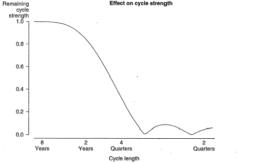
In the first step, cycles too short to be of interest would be separated out by applying a 7-term Henderson filter to seasonally adjusted constant price GDP(A). Chart 1, otherwise known as the gain function of the filter, shows the effect of this step on the strength of the various cycles in seasonally adjusted constant price GDP(A). The graph displays the various cycle lengths on the horizontal axis (logarithmic scale), and the proportion of the cycle that remains in the series after application of the filter, in this case a 7-term Henderson filter, on the vertical axis. It can be seen that the application of a 7-term Henderson has damped the effect of cycles of less than 4 quarters in length by at least two-thirds.
Chart 1. 7-TERM HENDERSON MOVING AVERAGE FILTER
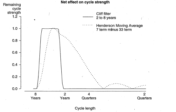
In the second step, cycles too long to be of interest would be separated out by applying a 33-term Henderson filter (H33) to seasonally adjusted constant price GDP(A). Chart 2 shows the effect of this step on the strength of various cycles, with cycles less than about 6 years being damped. The dotted line in Chart 3 shows the net effect of combining of these two filtering steps (footnote 6) (that is, Chart 1 minus Chart 2). It is apparent that this procedure, based on the Henderson filters, allows only approximate extraction of the 2 to 8 year frequency band. There are "ramps" or "shoulders" in the gain function. This may be contrasted with the "cliffs" in the gain function for a hypothetical filter that would extract precisely the 2 to 8 year band (shown by the solid line in Chart 3).
Chart 2. 33-TERM HENDERSON MOVING AVERAGE FILTER
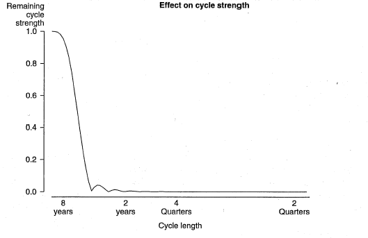
Chart 3. CLIFF AND HENDERSON MOVING AVERAGE FILTER
Of course, such "ramps" may be judged more desirable than the precise specification of a frequency band, because for example:
- an individual user may be unsure of how best to specify the length of the business cycle; or
- different users may disagree on how to specify the length of the business cycle; or
- the length of the cycle may be evolving.
In these circumstances, the Henderson-based procedure for estimating the business cycle may satisfy a broader range of users or acknowledge the uncertainties about the length of the business cycle. However, the remainder of this article assumes that users do wish to extract a given frequency band precisely.
TAILORED FILTERS
Recently, the ABS has developed "cliff" filters tailored to the task of extracting specified frequency bands from time series. The Appendix provides a more technical discussion of the construction and properties of such filters.
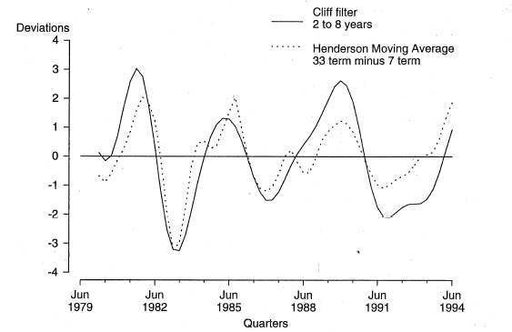
As an example of the application of this technique, Chart 4 contrasts two filtered forms of the GDP(A) series, intended to extract the "business cycle". The dotted curve shows the net result of applying the 33-term and 7-term Henderson filters. The solid curve shows the result of applying a filter tailored to extract precisely the 2 to 8 year frequency band. It can be observed that the double turns in 1983 and 1987 resulting from applying the H7-H33 filter disappear when the tailored filter is applied; also, there are some minor shifts in the timing of turning points. The choice between these two filtered versions of GDP(A) would depend in part on how sure the analyst is of the length of the business cycle and on what auxiliary information may be available concerning the trajectories of economic expansions and contractions; for example, there may be information to suggest that a double turn has occurred.
Chart 4. GDP(A) DEVIATION FROM LONG-TERM TREND
Using tailored filters, it is possible for the analyst to extract any desired combination of frequency bands. For example, instead of extracting all cycles between 2 and 8 years, an analyst may wish to extract for example cycles of 2-3 years, or 3-4 years etc. These are called one year slivers. Chart 5 shows the cycles when the tailored filter is applied to one-year slivers of GDP(A). The vertical scale shows the relative strengths of the slivers, in terms of deviations from the long-term trend. This decomposition may prove useful when the analyst wishes to construct forecasts of GDP(A) using leading indicators.
Chart 5. ONE YEAR SLIVERS OF GDP(A)
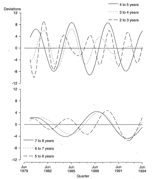
Table 1 shows the relative strengths of the cycles corresponding to one-year slivers for GDP(A) and 8 other economic indicators (the 8 components of the ABS's experimental Composite Leading Indicator). For example, for GDP(A) the cycle range 4 to 5 years represents 33 per cent of the sum of the variances of the slivers in the business cycle range (5 quarters to 8 years). This sort of analysis can be useful in understanding the cyclical signals given by various leading indicators. While none of the eight leading indicators in Table 1 shows precisely the same frequency composition as the reference series GDP(A), when taken together they represent the cycles present in the reference series. Some other selections of leading indicators could give poor forecasting performance: this could occur, for example, if the reference series showed considerable strength in a frequency band not represented or under represented among those leading indicators.
Table 1: RELATIVE PROPORTIONS OF THE VARIANCE OF CYCLES FOR THE PERIOD MARCH QUARTER 1980 TO JUNE QUARTER 1994
|
 | Years | |
 |
| 5 Quarters |
 | 7-8 | 6-7 | 5-6 | 4-5 | 3-4 | 2-3 | to 2 years |
|
| GDP (A) | 9 | 7 | 7 | 33 | 12 | 20 | 13 |
| Real interest rates | 2 | 5 | 17 | 12 | 4 | 21 | 38 |
| Trade factor | 16 | 11 | 25 | 20 | 15 | 7 | 4 |
| USA GDP | 14 | 6 | 17 | 22 | 8 | 26 | 6 |
| Job vacancies | 12 | 7 | 6 | 36 | 20 | 12 | 8 |
| Housing finance commitments | 6 | 9 | 10 | 39 | 17 | 7 | 10 |
| AII Industrials index | 10 | 14 | 9 | 1 | 8 | 41 | 18 |
| Production expectations | 4 | 4 | 4 | 16 | 30 | 22 | 21 |
| Business expectations | 3 | 3 | 4 | 15 | 39 | 22 | 15 |
|
| Note: Each entry shows the variance of the series in the one-year cycle range relative to the sum of the variances in the business cycle range (5 quarters to 8 years). |
Matching the frequency composition of the reference series is, of course, not the only criterion for constructing a composite indicator, because it reflects only the average "cyclical conformity" with the reference series, and does not guarantee early detection of particular peaks and troughs. For example, even if it were possible to find an individual indicator that showed an exact match with the frequency composition of GDP(A), it would still be wise to form a composite of several indicators.
Composite leading indicators have been found to be more robust in providing early warning of peaks and troughs. Cyclical fluctuations in the economy can be due to a wide variety of causes (for example, the weather, natural disasters, overseas and local events). Aggregating individual leading indicators into a composite indicator broadens the coverage of such causes and improves the prospect of detecting each peak and trough. Nevertheless, examining the frequency composition of both the reference series and candidates for components is a useful tool in the process of selecting components.
An advantage of tailored filters is that they allow exact extraction of a frequency band rather than an approximation thereto. However they have the disadvantage in that they require long-range backcasting and forecasting of the time series, as outlined in the Appendix.
CONCLUSION
Many varieties of economic analysis are assisted by filtering time series data to extract the signal (the cyclical component of interest). In the ABS's experience, the Henderson filters, which underlie the trend estimates that appear in many economic indicator publications, constitute a family of robust and adaptable tools for signal extraction. Recently, the ABS has been investigating and implementing methods of constructing filters that satisfy the more specialised needs of some analysts. For more information on the properties of Henderson filters and commonly used methods of analysing time series data, refer to A Guide to Interpreting Time series - Monitoring "Trends" (ABS Cat. No. 1349.0); for more information on tailored filters, contact the ABS Time Series Consultancy on (02) 6252 7646.
FOOTNOTES
- Key technical terms used in this article are explained in the Glossary below.
- A classic definition of the business cycle (attributed to Wesley C. Mitchell and quoted in OECD [1987]) is as follows "Business cycles are a type of fluctuation found in the aggregate economic activity of nations that organise their work mainly in business enterprises: a cycle consists of expansions occurring at about the same time in many economic activities, followed by similarly general recessions, contractions and revivals which merge into the expansion phase of the next cycle; this sequence of changes is recurrent but not periodic; in duration business cycles vary from more than 1 year to 10 or 12 years; they are not divisible into shorter cycles of similar character with amplitudes approximating their own."
To illustrate the application of tailored filters, this article has defined the business cycle as the 2 to 8 year frequency band; however, as explained in the section titled Tailored Filters, filters can be designed to extract any frequency band specified by the user.
- Year-apart movement - calculating the growth of the current period from the same period a year ago; for example, in trend terms, GDP(A) rose 4.6 per cent from the December quarter 1993 to the December quarter 1994; Moving annual sums - summing the data over a twelve month period; if the latest available trend estimate of GDP(A) is the December quarter 1994 estimate, the latest moving annual sum is the sum of the four latest quarterly estimates: March, June, September, and December quarters 1994.
- Henderson filters were first published in 1916 by Robert Henderson in Transactions (Actuarial Society of America) Volume 17 - "Notes on Graduation by Adjusted Average".
- The precise phase shift induced at the end points depends in part on the cycles present in the series being filtered.
- This procedure is used by the ABS to obtain the reference cycle for the experimental CLI.
GLOSSARY OF TECHNICAL TERMS
Time series - a sequential set of observations (or a statistical record), taken at regular intervals of a particular economic or social activity.
Filter, moving average - a transformation of time-series data to isolate certain frequencies.
Frequency - the number of occasions a cycle repeats within a given period.
Wavelength - the amount of time between successive repetitions of a cycle.
Amplitude - half the vertical difference between peak and troughs.
Gain - the change in amplitude of a series, after the application of a filter
GDP(A) The average of the three measures of GDP (the income approach, the production approach, the expenditure approach). GDP is defined as the total market value of goods and services produced in Australia, less intermediate consumption, but before allowing for the consumption of fixed capital.
APPENDIX - CONSTRUCTION AND PROPERTIES OF TAILORED FILTERS
Outline of the mathematics
Many filters, including the Henderson moving averages, were constructed to conform with desired smoothing and tracking criteria. See Chart 4 which shows quarterly GDP(A) graphed in the so-called "time domain" (ie, with time on the horizontal axis); filters can be constructed to remove such-and-such a proportion of short-term fluctuations from the series (smoothing) and to ensure that the filtered series replicates such-and-such key features of the path taken by the original series (tracking). Although it is possible to choose, say, a Henderson filter that will partially damp specified frequencies, the effects on component cycles of various frequencies are side-effects of the filter design.
It is possible, however, to design filters directly to conform with desired criteria expressed in terms of the so-called "frequency domain". The solid line in Chart 3 shows the design criterion for a filter that exactly reproduces cycles in the two-to-eight year frequency band and eliminates all other cycles from quarterly time series. The mathematical tool for constructing such filters is the Fourier transform. However, standard Fourier methods yield filters exhibiting quite erratic convergence of the gain to the desired "cliff" shape; ABS research has led to modifications that yield a set of filter weights ensuring smooth converge of the gain to the desired shape. These weights are computed using the following formula:
For 2 * m + 1 symmetric weights to give a "cliff" at frequency f
W0 = 1 / PI * (f + 0.5 * (e2 - e1))
Wj = c2/ PI * [ sin(( f + e2 ) * j ) + sin(( f - e1) * j ) ] / [2 * j * ( c2- j2 )]
for j=1,m
where c = PI / (e1 + e2) and e1 and e2 are suitably chosen constants.
Outline of forecasting and backcasting methods
This technique of filter construction demands a long run of data - much longer than the typical economic time series published by the ABS. Hence data are backcast and forecast; these extensions need not be accurate provided they capture essential features of the data. Two methods of backcasting/forecasting a series that have been investigated so far are to use:
- a common autoregression (AR) model that captures the essential features of a group of data series (eg, the ABS's employment series). The filtered data at the end of the series can be viewed as the result of an amalgamation of model-based and model-free approaches to filter design.
REFERENCES
- OECD 1987, OECD Leading Indicators and Business Cycles In Member Countries 1960-1985, OECD Sources and Methods, No. 39
- Australian Bureau of Statistics, A Guide to Interpreting Time Series - Monitoring "Trends" (ABS Cat. No. 1349.0)
|
 Print Page