APPENDIX 2 JUSTIFICATION AND TEST RESULTS


ADAPTATION OF MULTILATERAL TESTS FROM VOLUME SHARES TO PRICE AND QUANTITY COMPARISONS

The tests for multilateral indexes presented by Diewert (1999) and Balk (2001) are expressed in terms of volume shares. These volume shares are equivalent to normalised quantity index levels, and can also be expressed in terms of prices, quantities and (multilateral) price levels:

(A.1)

Where is the volume share in period , and are price and quantity vectors respectively in period and is the multilateral price level in period t.

Test 1 states that are positive and continuous and normalised so that

(A.2)

This implies that the quantity comparison between any pair of entities (e.g. time periods) and ,

(A.3)

is also positive and continuous.

The product test states that

(A.4)



where and are the expenditure and price comparisons respectively between periods and .

Moreover the expenditure comparison can be expressed as:

(A.5)

These expenditure comparisons are also positive and continuous. In consequence, the price comparisons are also positive and continuous. For multilateral temporal price comparisons, it is customary to normalise the price index levels such that:



Several Tests, including 2, 2x, 2p, 3, 4, 11, and the first part of Test 8, can easily be expressed in terms of quantity comparisons, and then A.4 and A.5 can be used to derive the implied Test for price comparisons after some simple algebra. In most cases the price comparison Test corresponds closely to the quantity comparison Test, with the possible exception of Test 11. This Test states that combining volume shares additively in each group yields a Fisher quantity index, which means that price levels need to be combined harmonically to yield a Fisher price index.

Derivations of all these tests are not shown here, but Test 3 is presented as an example. Define as the set of original price vectors, as the set of original quantity vectors, and as the set of quantity vectors after rescaling by a positive constant in an arbitrary period . Then homogeneity in quantities implies that:

(A.6)

Using A.5, it is easy to show that:

(A.7)

Substituting A.6 and A.7 into A.4, it follows that:

(A.8)

In other words, Test 3 implies that price comparisons should be unaffected by scaling the quantity vector in any period if prices do not change.

Tests 5, 6, 7 and the second part of Test 8 state that the volume shares are invariant to changing the units of measurement, reordering the time periods, reordering commodities, or aggregating/disaggregating other entities. None of these changes alters expenditure comparisons, so tests that they do not alter volume shares are equivalent to tests that they do not alter price comparisons (this follows from the product Test A.4).

Test 9 states that a time period's influence on quantity comparisons between other periods vanishes as the magnitude of its quantity vector approaches zero. Under the same condition, the time period's influence on price comparisons between other periods must vanish as well. This suggests that Test 9 is inconsistent with Test 3.

Test 10 states that each period's volume share is an increasing function of its quantities, which implies that is an increasing function of the elements of . A corresponding and appealing Test for price comparisons would be that is an increasing function of the elements of , but this doesn't seem to follow from Test 10.

Finally, Balk (2001: section 4) clearly describes formulae for the price and quantity indexes under an additive multilateral method, so there is no need to derive these here.


JUSTIFICATION OF NEW TEST RESULTS

Most of the Test results in Table 4.2 are assessed by Diewert (1999) and/or Balk (2001). However, a few combinations of tests and methods are not assessed, including

• The TPD method's satisfaction of Tests 10, 11 and 12;
• The QAUV_TPD method's satisfaction of any of these Tests;
• Whether these Tests are preserved for extended multilateral indexes.

A brief justification of the corresponding claims in Table 4.2 is appropriate here. We do not present formal mathematical proofs but focus on the reasoning behind each claim; verification of the details is left to the reader.


TPD

The TPD's performance against Tests 10 and 11 is not evaluated here. Test 11 is not critical for this publication, though it seems unlikely that the TPD would satisfy it, given the bilateral TPD index's similarity to the Törnqvist index as opposed to the Fisher index. However, as noted by both Balk (2001) and Rao (2005), the TPD is equivalent to the Rao method, which is not additive (fails Test 12).


QAUV_TPD

The QAUV_TPD satisfies Test 1, since quantity comparisons can be expressed as:

(A.9)

where

and both the quantity vectors and (derived from a TPD model) are positive and continuous.

If for every , then from A.9

(A.10)

so the QAUV_TPD satisfies Test 2x. Similarly, if prices are proportional then the vector derived from the TPD model satisfies for every , since the TPD satisfies Test 2p (this equality can be verified through examining the equations defining the Rao method, which is equivalent to the TPD). It follows that:

(A.11)

so the QAUV_TPD satisfies Test 2p. As Balk (2001) notes, satisfaction of either Test 2x or 2p is sufficient to guarantee satisfaction of Test 2.

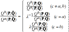
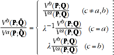
Scaling the quantities in some period does not alter , as the TPD model uses expenditure share weights. Examination of A.9 reveals that the quantity comparisons satisfy equation A.6 provided is not altered, so the QAUV_TPD satisfies Test 3.

Similarly, scaling the prices in some period does not alter , so the QAUV_TPD satisfies Test 4. To verify this, define ; it is easy to show that:

(A.12)

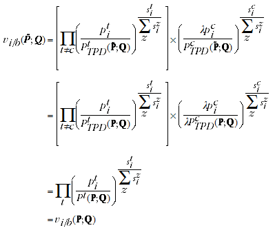
And using the expression for the reference prices/quality adjustment factors in the Rao method (equivalent to the TPD):



where the first equality holds due to A.12, and the second equality holds(footnote 1) because the TPD satisfies Test 4. The QAUV_TPD satisfies Test 5 because

(A.13)

where is an NxN diagonal matrix expressing the change in units of measurement for each commodity. It is easy to show that multiplying each price vector by also inflates in the same way (when expenditures do not change) using logic similar to the justification of Test 4.

The QAUV_TPD method satisfies Tests 6 and 7 because the TPD satisfies these Tests. Similarly, the QAUV_TPD fails Test 9 because the TPD fails this Test, so the prices in a time period continue to influence even as the quantities sold in that period approach zero.

The QAUV_TPD method's failure of Test 8 derives from the expenditure share weighting used in the TPD: splitting or aggregating across periods in a group alters the weights given to those periods' prices in deriving the , hence it alters the QAUV_TPD comparisons between other periods.

As with the TPD, the QAUV_TPD is not formally assessed against Tests 10 and 11 here (though it seems unlikely to satisfy Test 11). Its additivity is clear from A.9.


Test performance of extended multilateral indexes

When the methods described in this publication are used to extend multilateral indexes, most price and quantity comparisons are not derived from a single multilateral window but by combining (multiplying or dividing) price movements from a series of partially overlapping multilateral windows. It is important to consider whether Tests satisfied by each multilateral index are preserved after we combine price and quantity comparisons in this way.

Test 1 is clearly preserved after extension - the result of multiplying or dividing positive and continuous functions is necessarily positive and continuous.

Tests 2, 2x and 2p state that if strong conditions hold within a multilateral window, there is a unique price and/or quantity comparison between each pair of time periods. It is easy to see that if these conditions hold in general, they also hold within each multilateral window (or vice versa), and that the unique price and/or quantity comparisons are transitive, so these Tests are preserved after extension.

Tests 3, 4 and 9 relate to the effect of scaling the quantities or prices in one period on the system of comparisons. Clearly, scaling the quantities or prices in that one period cannot affect the system of comparisons in a window that does not contain it. It follows that if these Tests hold within windows containing the period, they hold in general.

Test 5 states that changing any product's units of measurement (across all time periods) should not alter the system of comparisons. So long as any changes in a product's units of measurement are constant across time, this invariance should be preserved after extension.

Test 6 states that reordering the time periods should not alter the system of comparisons, which may be true within each multilateral window but not for an extended index. For instance, suppose we have two windows that overlap in at least two periods ( and ) and that a third period ( ) is in one window but not the other. Due to the influence of price and quantity information from period , the two multilateral windows will in general yield different comparisons between periods and . How each extension method forms the multilateral windows and derives the definitive price movement between a and b (from these and/or other windows) depends on the temporal ordering; so reordering the time periods (or changing the way the index is extended) may alter the extended index values.

Test 7 states that reordering the commodities should not alter the system of comparisons. Although the methods used to extend the index depend on the temporal ordering, they do not depend on the order of commodities, so this property is preserved after extension.

Additivity means that quantity comparisons can be expressed in the form of A.9. As noted above, most of the quantity comparisons in the extended index are derived by combining (multiplying or dividing) quantity comparisons from individual multilateral windows. It can be shown that, even if the multilateral comparisons within each window are additive, the full system of extended comparisons (products or quotients of additive comparisons) cannot be expressed in the form of A.9 unless the vectors from every multilateral window (or the quantity vectors in every time period) are proportional to one another. Neither of these conditions holds in general, so Test 12 fails. However, if there is substantial overlap between two windows, the vectors from each window are likely to be approximately equal, so short term index movements should approximate an additive index closely. Tests 8, 10 and 11 need reinterpretation for temporal comparisons, so the performance of extended indexes against these Tests in their current form is not critical for this publication. That said, it would appear that Test 8 at least does not hold for extended indexes, as aggregating or disaggregating time periods would affect the temporal sequencing that is used in updating the index level; and Test 11 seems likelier to be preserved, based on logic similar to the justification of Test 2 (since the conditions imposed on the price and quantity vectors are similar).

1 Up to the choice of a TPD normalisation factor, which would cancel out of the QAUV_TPD comparisons. <back