Page tools:
 Print Page Print Page
 Print All Print All
| |||||||||||||||||||||||||||||||||||||||||||||||||||||||||||||||||||||||||||||||||||||||||||||||||||||||||||||||||||||||||||||||||||||||||||||||||||||||||||||||||||||||||||||||||||||||||||||||||||||||||||||||||||||||||||||||||||||||||||||||||||||||||||||||||||||||||||||||||||||||||||||||||||||||||||||||||||||||||||||||||||||||||||||||||||||||||||||||||||||||||||||||||||||||||||||||||||||||||||||||||||||||||||||||||||||||||||||||||||||||||||||||||||||||||||||||||||||||||||||||||||||||||||||||||||||||||||||||||||||||||||||||||||||||||||||||||||||||||||||||||||||||||||||||||||||||||||||||||||||||||||||||||||||||||||||||||||||||||||||||||||||||||||||||||||||||||||||||||||||||||||||||||||||||||||||||||||||||||||||||||||||||||||||||||||||||||||||||||||||||||||||||||||||||||||||||||||||||||||||||||||||||||||||||||||||||||||||||||||||||||||||||||||||||||||||||||||||||||||||||||||||||||||||||||||||||||||||||||||||||||||||
These fact sheets provide a broad overview of the key concepts and data sources for measuring household economic wellbeing. The Household Economic Wellbeing fact sheet series currently comprises:
The series may be expanded in the future to cover other aspects of these important statistics. FACT SHEET 1. WHAT IS HOUSEHOLD ECONOMIC WELLBEING? When considering the circumstances of households, the key economic wellbeing factors that affect people's material standard of living are income, consumption and wealth. Income can be used to support consumption of goods and services, such as food, clothing, housing and leisure activities. Alternatively, it can be saved and invested to increase wealth which can be used at a later date to support consumption. Some people with low incomes have considerable wealth allowing them to maintain consumption levels above their current income. People with low reserves of wealth may face financial difficulty in times of need, such as during any period of reduced income or substantial unexpected expenses. Diagram 1 illustrates this relationship, although people's actual wellbeing is affected by individual circumstances and lifestyle choices. Diagram 1. Components of economic wellbeing
Income levels and wealth vary over a person's life and are affected by two main factors, age and labour force participation. Incomes tend to grow until middle age. Wealth tends to be gradually accumulated during the working lives of household members and used during retirement. (Graphs 1 and 2) 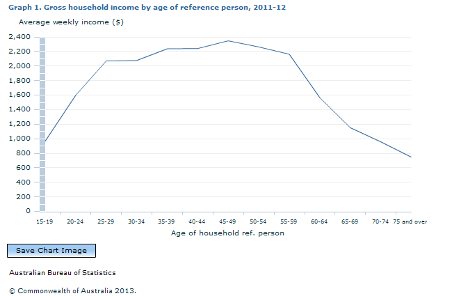 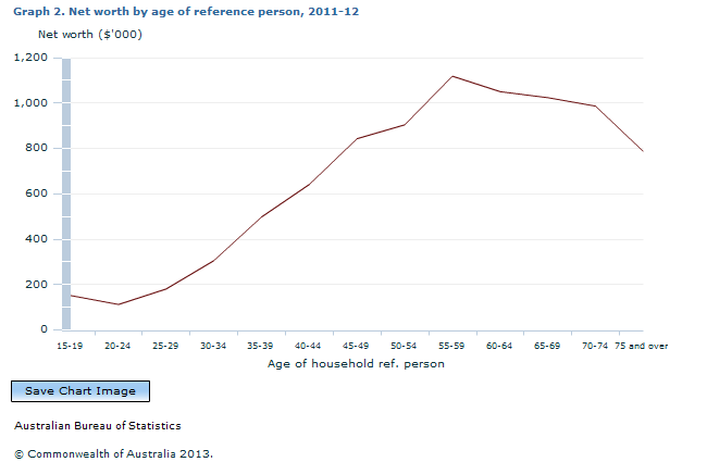 Key concepts for measuring economic wellbeing The definitions used to measure the economic wellbeing of people can have a significant impact on the results. The Australian Bureau of Statistics (ABS) follows international best practice in producing micro statistics relating to household economic resources. Income The most comprehensive measure of income is compiled from the ABS Survey of Income and Housing (SIH) and the ABS Household Expenditure Survey (HES). This definition aligns with new international standards released in 2004 and fully adopted from SIH 2007–08 and HES 2009–10:
The first international wealth standards were published by the OECD in 2013.
Consumption expenditure The international definition of consumption expenditure is summarised as:
In the HES, expenditure is valued as the cost of goods and services acquired during the reference period for private use, whether or not the goods were paid for or consumed in that period. Expenditure is net of refunds and trade-ins. Consumption expenditure includes in kind income from employers, such as subsidised housing or the use of a car for private purposes. Broadening the income measure In recent years the ABS has made significant progress in extending its measurement of household income to reflect real world changes and enhance analytical opportunities. This includes developing new measures to allow the full economic circumstances of different types of households to be compared. In particular, the ABS has produced:
b) social transfers in kind (STIK) allocations from SIH 2011–12 (previously only based on HES data) c) final income estimates since 1984. What is it? Income from imputed rent is allocated to owner occupiers and households living in subsidised private rentals e.g. renting from a family member. For owner occupiers, income from imputed rent is the estimated market rent of a dwelling less housing costs normally paid by a landlord such as mortgage interest, rates, insurance and repairs. For renters, it is the difference between market rent and actual rent paid. Why include imputed rent in income? Housing is one of the most significant living costs borne by many households. The inclusion of imputed rent in income provides a broader picture of the economic wellbeing of owner occupied and rent-subsidised households relative to other households, allowing more meaningful comparisons of the wellbeing of people living in different tenure types.b) Social transfers in kind What are they? Social transfers in kind are goods and services provided by governments that benefit individuals but are provided free or at subsidised prices. Examples include free or subsidised education, health and child care. Why include STIK in income? STIK have a significant impact on the wellbeing of people and on the measurement of the distribution of income. This is important for comparisons within and across countries. In Australia, many government services have been designed to assist those most in need of financial support. The allocation of benefits differs between households, reflecting characteristics such as household composition, life cycle stages, household size and income. The inclusion of IR and STIK increased the mean equivalised disposable household income (EDHI) from $918 to $1220 per week in 2011–12 and reduced the inequality of income distribution across households. (Graph 3) Graph 3. Distribution of equivalised disposable household income with and without IR and STIK, 2011-12 Source: ABS Survey of Income and Housing (6523.0) Appendix 4 Social transfers in kind c) Final incomeWhat is it? Final income is equal to household private income plus social assistance benefits in cash (e.g. age and disability support pensions, Family Tax Benefit) and STIK less income taxes and taxes on production (e.g. GST and taxes on alcohol and cigarettes). Both household income and expenditure are required to estimate final income. This data is available whenever the HES is conducted, most recently in 2009–10. (Diagram 2) Why is it important? Final income shows the full effect of government expenditure and taxes on the distribution of income among private households in Australia. This allows policy makers to understand the effects of changes in either government revenues or spending that directly impact on the economic wellbeing of households. The net effect of government benefits and taxes in 2009–10 was to increase average incomes of households in the three lowest quintiles and decrease those of the two highest quintiles. (Graph 4) 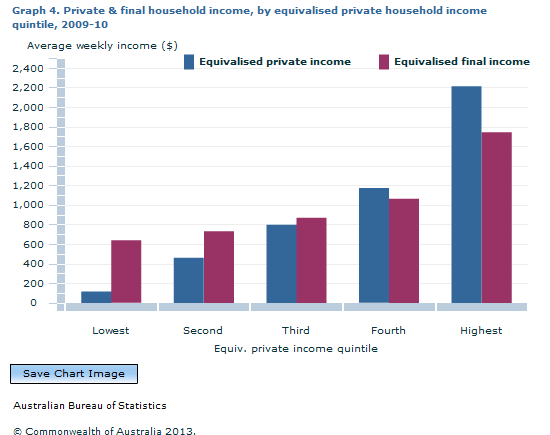 Diagram 2 illustrates the relationship between the different income concepts presented in this Fact Sheet Series. Diagram 2. Income concepts and components FACT SHEET 2. UNDERSTANDING MEASURES OF INCOME AND WEALTH Why is income and wealth distribution important? Economic and social analysts and policy makers are interested in the distribution of resources and how this affects the wellbeing of society and individuals, particularly people's ability to acquire the goods and services required to satisfy their needs. Questions that researchers ask include:
Why is an equivalence scale used? As household size increases, consumption needs also increase but there are economies of scale. An equivalence scale is used to adjust household incomes to take account of the economies that flow from sharing resources and enable more meaningful comparisons across different types of households. For a lone person household equivalised income is equal to actual income. For households comprising more than one person, it is the estimated income that a lone person household would need to enjoy the same standard of living as the household in question. How are equivalising factors calculated? Equivalising factors are calculated based on the size and composition of the household, recognising that children typically have fewer needs than adults. The ABS uses the OECD-modified equivalence scale which assigns a value of 1 to the household head, 0.5 to each additional person 15 years or older and 0.3 to each child under 15 years. Table 1 shows that a couple household with one child would need $1,800 weekly disposable income to have the same equivalised disposable household income (EDHI) as a lone person household with a disposable income of $1,000. Table 1. Examples of equivalised weekly disposable household income
Equivalence scales used for household income are equally applicable for consumption measures. There is less agreement about how to equivalise household wealth as wealth is often built up during a person's working life and then used during retirement when the composition of the household might be quite different. However, when wealth is being used to support current consumption, particularly for households at risk of economic hardship, household wealth should be equivalised with the same scale used to equivalise household income and consumption. Analysis of households and persons There are two common ways of presenting analysis of households:
To provide a better understanding of the circumstances of people it is often preferable to study people in households e.g. the number of people in Australian households experiencing economic hardship. In this analysis, each person is attributed with the characteristics of the household to which they belong, e.g. household income is used to determine whether it is a low or high income household but analysis is about numbers of people experiencing hardship. This approach keeps the focus on individual circumstances while recognising that people share household resources. Summary measures There are several summary measures commonly used for analysing household economic wellbeing. Counts Counts provide an estimate of the total number of people or households with a particular characteristic and are derived by summing the survey weights of each observation of interest. In sample surveys the weights enable extrapolation of the survey responses to official population estimates. Means The arithmetic mean, or average, is the sum of all income divided by the number of observations. Advantages of the mean are that it is easy to calculate and the means of all subcomponents sum to the mean of all observations. Its drawbacks are the effect of extreme values and asymmetry of the distribution, both of which are relevant for income and wealth data. For example, a small number of very wealthy and a large number of relatively poor households may have the same average income or wealth as a population where there is equal distribution of resources. Medians Medians are calculated by ranking all observations from the lowest to the highest. The middle observation of the distribution is the median. Compared to the mean, the median is a more stable measure and is less affected by extreme values and sample fluctuations. However, median values of subcomponents do not add up to the median of all observations. Distribution measures Measures of the distribution of income and wealth help to describe and understand how economic resources are shared across the population and households. Frequency distribution Frequency distributions show the proportion of people or households with a particular level of income or wealth. To produce the distribution, the item of interest is ranked by value and the population grouped into classes. The ABS currently uses $50 ranges for weekly income and $100,000 ranges for wealth. It is useful to include the summary statistics such as the mean and median in the frequency distributions. Income and wealth distributions tend to be asymmetrical, with a small number of people having relatively high income or wealth and a much larger number having relatively low income or wealth. (Graph 1)Graph 1. Distribution of equivalised disposable household income, 2011-12 Source: ABS data available on request, Survey of Income and Housing (6523.0) Quantiles Quantile is a term for groups formed by ranking the units of analysis (e.g. household or persons) in ascending order and calculating the shares of the total accruing to a given proportion of the units:
, by quintile, 2011-12.gif) Source(s): ABS Survey of Income and Housing (6523.0) Percentile ratios The boundary between quantiles is usually expressed as the upper value of a particular percentile. The ABS publishes the upper value of each decile (P10 to P90). This provides the range of values in each quintile, e.g. the middle (3rd) quintile is formed by households with income/wealth between P40 and P60. The median of each quintile can also be determined, e.g. the median of the first quintile is P10, second quintile, P30, etc. The median of the whole population is P50. Percentile ratios summarise the relative distance between two points on the income or wealth distribution. Percentile ratios will be less volatile than measures based on means, particularly at each end of the distribution. To illustrate the full spread of the income distribution, the percentile ratio should use points near the extremes e.g. the P90/P10 ratio. The P80/P20 ratio better illustrates the magnitude of the range for the majority of the population. The P90/P50 and P10/P50 ratios compare the ends of the distribution with the median and these are commonly used to understand how the wealthier compare to average and the poorer to average. Table 2 shows that income is more equally distributed than wealth. In 2011–12, the equivalised income of households at the top of the 80th percentile (or fourth quintile) was 2.6 times higher than that of households at the top of the 20th percentile (or lowest quintile), whereas wealth was 10 times higher (P80/P20). Table 2. Ratio of values at top of selected percentiles, 2011–12
Shares of income or wealth Income or wealth shares can be calculated and compared for each quantile of a population. The aggregate income/wealth of units in each quantile is divided by the total aggregate of the entire population to derive quantile share. Graph 3 shows income and wealth shares by decile. Household wealth is more unequally distributed than household income. People in the three lowest equivalised income deciles received 13% of all income, whilst people in the three lowest equivalised wealth deciles held only 3% of all wealth in 2011–12. , 2011-12.gif) Footnote(s): (a) Decile boundaries are derived separately for equivalised disposable income and net worth Source(s): ABS Survey of Income and Housing (6554.0) Gini coefficient The Gini coefficient is a single statistical indicator of the degree of inequality. It equals zero when all people have the same level of income and equals one when one person receives all the income. In general the smaller the Gini coefficient, the more equal the distribution of income or wealth. Any increase in the income of a person with income greater than the median will always lead to an increase in the Gini coefficient, while an increase in the income of a person with income lower than the median will always lead to a decrease in the coefficient. The distribution of income becomes more equal when imputed rent and social transfers in kind (STIK) are included in the income measure, down from 0.320 to 0.226 in 2011–12. (Table 3) Table 3. Gini coefficient, by household income, 2011–12
Measurement ErrorsSampling Error Household survey estimates are based on a sample of possible observations and are subject to sampling variability. The sampling error is a measure of the variability that occurs by chance because a sample, rather than the entire population, is surveyed. One measure of the likely difference is given by the standard error (SE). Another measure of the likely difference is the relative standard error (RSE), which is obtained by expressing the SE as a percentage of the estimate. The RSE is a useful measure in that it provides an immediate indication of the percentage errors likely to have occurred due to sampling, and thus avoids the need to refer also to the size of the estimate. The ABS annotates estimates with a RSE between 25% and less than 50% by a preceding asterisk (e.g. *3.4) to indicate they are subject to high SEs and should be used with caution. Estimates with RSEs of 50% or more are preceded with a double asterisk (e.g. **0.6), indicating that these estimates are considered unreliable for most purposes. Significance Testing To compare estimates between surveys or between populations within a survey it is important to determine whether apparent differences are 'real' differences between the corresponding population characteristics or simply the product of differences between the survey samples. A common approach is to determine whether the difference between the estimates is statistically significant by calculating the standard error of the difference between two estimates (x and y) and using that to calculate the test statistic using the formula below: If the value of the statistic is greater than 1.96 there is good evidence of a statistically significant difference at 95% confidence levels between the two populations for the characteristic being tested. Otherwise, it cannot be stated with confidence that there is a real difference between the populations. FACT SHEET 3. LOW ECONOMIC RESOURCE HOUSEHOLDS People living in low economic resource households are of particular policy and research interest because of their greater risk of experiencing economic hardship. This fact sheet summarises different methods available to identify these households and provides guidance on methods of analysing them. There are many factors influencing whether people are experiencing economic hardship. The analysis of household economic wellbeing is enhanced significantly when the income, consumption and wealth dimensions are studied jointly, recognising they vary over the lifecycle:
Composite measures of low economic resource households Low economic resource measure Diagram 1. Low economic resource households The ABS has developed a low economic resource measure (LER) that includes people who are simultaneously in the lowest four deciles of both equivalised disposable household income (EDHI) (including imputed rent) and equivalised household net worth (LER40). This measure therefore excludes people with either relatively high incomes or relatively high wealth. As a result it is more likely to correctly classify people at risk of experiencing economic hardship compared to measures using income or wealth alone. The LER is a relative measure that classifies around 20% of people in low income, low wealth households. It does not identify whether these people are actually experiencing economic hardship. The actual proportion will vary over time as the joint distribution of income and wealth changes. One of the strengths of this measure is its ability to contrast the characteristics of the LER population with those in the low income and low wealth quintiles. Table 1 compares selected characteristics of LER households to households with low income or low wealth only. The proportion of couple or lone person households where the reference person is 65 and over, reduces from 28% of low income households to 6% of LER households, reflecting their ability to draw on accumulated wealth. In contrast, whilst 35% of low income households are private renters, this group accounts for 52% of LER households. Table 1. Persons in low economic resource households, 2011–12
(a) Persons in the lowest two deciles of EDHI (incl. imputed rent) (b) Persons in the lowest two deciles of equivalised household net worth (c) Persons in the lowest four deciles of both EDHI (incl. imputed rent) and equivalised household net worth Source: ABS Survey of Income and Housing (6523.0) Feature Article: Low Economic Resource Households Other composite measures of economic hardshipThe LER measure can be broadened by considering experiences of 'financial stress' or 'missing out'. The indicators used to define these measures are listed in Table 3 of this fact sheet. Graph 1 shows examples of LER measures by:
Graph 1. Measures of low economic resource households, proportion of persons, 2009-10 Source: ABS data available of request, Household Expenditure Survey (6530.0) Single dimension measurement of household economic wellbeing When measuring economic wellbeing it is preferable to consider multiple dimensions, particularly income and wealth, however both measures are not always available. This section describes several commonly used single dimension measures of economic wellbeing. Income Income is the most frequently available measure of economic wellbeing. For most households, it is the main resource used to meet daily expenses. However, analysis using income alone has significant limitations. Income can be volatile for people who are making transitions between study, jobs, into retirement or changing their hours of work e.g. to care for children. At these times, households may draw on other resources, such as using savings or increasing their debt. Being able to identify households with accumulated wealth to supplement low incomes is desirable as these people are less likely to experience economic hardship than households without alternative resources to fall back on. a) Relative poverty measures based on income Many developed countries use relative poverty to measure the economic wellbeing of households. These measures identify the proportion of people with an income below a certain fraction of median EDHI. The OECD publishes various analyses based on poverty lines below 40%, 50% or 60% of median incomes (50% used most often), while Eurostat commonly uses 60% as the cut-off. Limitations of relative poverty measures include:
Table 2. Relative poverty measures based on proportion below a percentage of median income, 2011–12
While it is tempting to label all households in the lowest income decile as ‘low income’, ABS analysis suggests there are variable economic circumstances for households in this group. Households with nil or negative income, or income below government pension rates, make up almost one half of the lowest income decile. However, more than 40% of households in the lowest income decile have net worth in the top five wealth deciles, suggesting a temporary setback to their economic wellbeing, such as a temporary loss in their business operations or a temporary job loss. 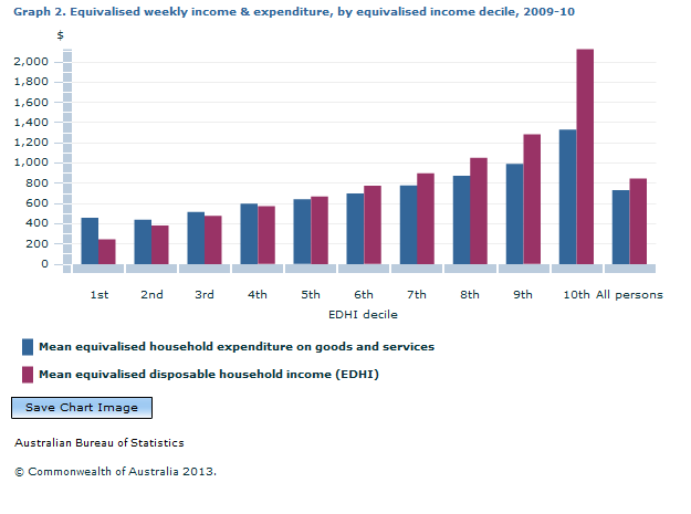 Furthermore, people in the lowest decile of EDHI had average equivalised expenditure higher than those in the second income decile in 2009–10. (Graph 2) The ABS therefore uses the second and third income deciles to describe 'low income' households rather than the lowest income quintile. However, as the lowest decile includes many households whose only source of income is a government pension or allowance, some people in the lowest income decile experience high levels of economic hardship. Therefore, for many analytical purposes a lower cut-off should be applied to only remove extreme low value households that may distort the results. In 2011–12, Age Pension rates (excluding supplementary payments) for singles and couples were around the 7th percentile of EDHI. Financial stress indicators While income and wealth statistics describe the economic resources available to people and expenditure statistics describe their consumption patterns, there are other issues relevant to understanding living standards e.g. a person with poor health and high health care costs may have reduced income for other purchases. In attempting to identify which households have the lowest economic wellbeing, other indicators of poor economic outcomes can be considered. Data relating to experiences of financial stress and missing out are collected in the HES. (Table 3) Table 3. Indicators of financial stress in the last 12 months
Financial stress information can provide insight into people’s economic wellbeing although analysis needs to consider overall circumstances. Some individuals may have consumption priorities which differ from socially accepted norms of the 'basics of life'. In 2009–10, 20% of households in the highest EDHI quintile reported at least one financial stress indicator. (Graph 3) 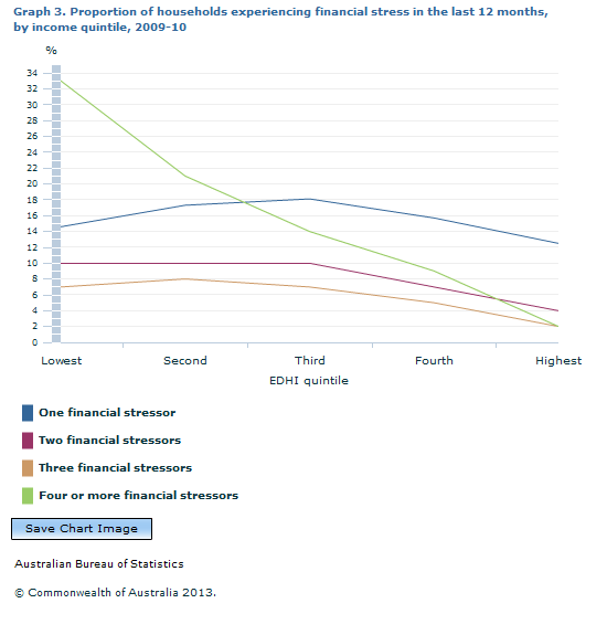 Source(s): ABS Household Expenditure Survey (6530.0) Measuring persistent economic hardship Another key policy interest is people experiencing long-term and persistent economic hardship as distinct from those experiencing short-term hardship. Longitudinal datasets, such as the Household Income and Labour Dynamics Australia Survey (HILDA) and the ABS Australian Census Longitudinal Dataset (ACLD), are important sources for identifying people experiencing long-term economic hardship. The HILDA has been tracking the economic circumstances of many respondents since 2001. The ACLD will provide a five-yearly snapshot of the income and housing circumstances of people from 2006. The SIH measures the short-term persistence of economic hardship by comparing income from the previous financial year with current year income. The circumstances of people with low incomes in both periods can be identified. Combined with wealth data which is more stable over time, this provides a more accurate picture of whether hardship is persistent. As well as financial stress experiences, the HES also collects data on people's perception of their current financial circumstances compared to two years ago and their ability to save money. FACT SHEET 4. KEY DATA SOURCES Key data sources There are many useful data sources providing information on the economic wellbeing among households in Australia. This fact sheet uses the ABS Data Quality Framework to provide information about the following key data sources (Tables 1 and 2):
Table 1. Key data sources
Table 1. Key data sources continued
Migrants The ABS produces a range of data on the economic wellbeing of migrants. This includes:
Disabled people and carers The Survey of Disability, Ageing and Carers (SDAC) is a cross-sectional survey conducted every three years in both private and non-private dwellings. Data are available for 1993, 1998, 2003, 2009 and 2012. Includes long-term health conditions and care requirements (including for older people), financial impacts on carers and income. The latest output is Disability, Ageing and Carers, Australia: Summary of Findings, 2012 (4430.0). A CURF will also be available in early 2014. Aboriginal and Torres Strait Islander peoples The National Aboriginal and Torres Strait Islander Social Survey (NATSISS) is a cross-sectional survey conducted every six years. Data are available for 1994, 2002 and 2008. Data are collected from Aboriginal and Torres Strait Islander peoples in private dwellings in both remote and non-remote areas, including income and finances, work, housing and mobility and financial stress.
Integrating administrative data to measure economic wellbeing Statistical data integration involves bringing together data from different sources at the unit level (e.g. for an individual person or organisation) or micro level (e.g. information for a small geographic area) to enable analysis of a combined set of information for statistical and research purposes. Analysis of integrated administrative and other data offers valuable opportunities to investigate more complex and expanded policy and research questions than would be possible using only separate, unlinked data sources. As the data is already collected for an administrative purpose, it can be used without imposing additional burden. Administrative datasets provide opportunities for both cross-sectional analysis of society, small areas and subpopulations of interest, along with longitudinal analysis of the circumstances of individuals, households or families. Diagram 1 shows how administrative data sources relate to the concepts of household economic wellbeing. Diagram 1. Household economic wellbeing measures and relationships based on administrative data FACT SHEET 5. CHANGES OVER TIME Changes in the levels and distribution of economic resources in a society over time are key concerns of social and economic analysts. This fact sheet presents time series analysis of the three dimensions of household economic wellbeing – income, consumption and wealth. The analysis uses data from the Survey of Income and Housing (SIH), Household Expenditure Survey (HES) and Household Income and Labour Dynamics in Australia Survey (HILDA). Income Income data has been collected in the HES since 1984 and in the SIH since 1994–95. Since 1994–95, median equivalised disposable household income (EDHI) has increased in real terms from $505 to $790 (up 56%). Low income households have had a slightly lower real increase in their average income (47% at top of P10) than high income households (60% at top of P90). (Graph 1) Graph 1. Equivalised disposable household income at top of selected percentiles, 1994–95 to 2011–12(a) (a) In 2011-12 dollars, adjusted using changes in the Consumer Price Index Source: ABS Survey of Income and Housing (6523.0) Average wages and salaries and government pensions and allowances both increased significantly in real terms between 1994–95 and 2011–12 (52% and 24%, respectively). The Gini coefficient is a single statistic between zero and one and is a summary indicator of the degree of inequality, with values closer to 0 representing less inequality, and values closer to one representing greater inequality. Since 1994–95, the Gini coefficient for EDHI has been lowest in 1996–97 (0.292) and highest in 2007–08 (0.336). It decreased by 5% between 2007–08 and 2011–12. (Graph 2)Graph 2. Gini coefficient of equivalised disposable household income, 1994–95 to 2011–12 Source: ABS Survey of Income and Housing (6523.0) The HILDA survey provides valuable insight into economic circumstances over time and the persistence of income disadvantage for individual households. Two thirds of households with a low income (lowest two income quintiles) in 2001 continued to have a low income in 2009. Similarly, over 60% of high income households (highest two quintiles) in 2001, remained at the top of the income distribution in 2009. (Graph 3)  Source(s): HILDA Families, Income and Jobs, Volume 7 Improvements in the SIH since 2003–04 The ABS has implemented improvements to the SIH to ensure the survey accurately measures the distribution of economic resources among households in Australia, including:2003–04
(a) In 2011-12 dollars, adjusted using changes in the Consumer Price Index Source: ABS Survey of Income and Housing (6523.0) Consumption expenditure As incomes have risen, consumption expenditure has also risen. Between 1984 and 2009–10 average weekly expenditure of all households increased in real terms by one third from $933 to $1,236. The increase in expenditure was greatest for households in the fourth and fifth gross income quintiles. In these quintiles average income exceeded average consumption expenditure by 14% and 31%, respectively in 2009–10. By comparison, households in the lowest two income quintiles had average expenditure higher than their average disposable income. (Graph 5) 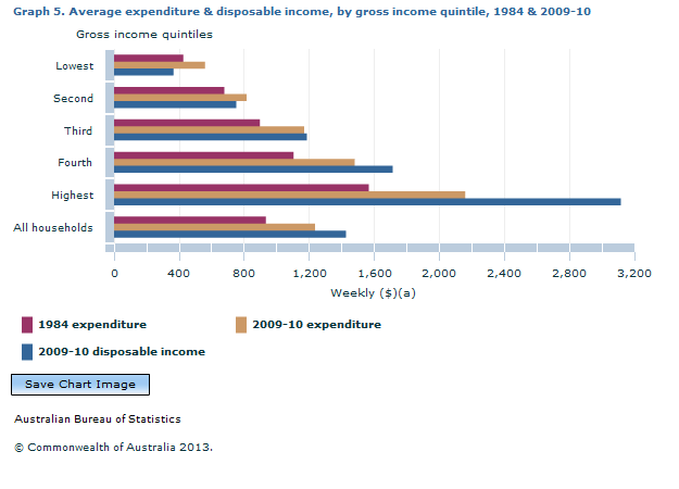 Footnote(s): (a) In 2009-10 dollars, adjusted using changes in the Consumer Price Index Source(s): ABS Household Expenditure Survey (6530.0) Consumption patterns of households have changed since 1984. Current housing costs increased from 13% of total household expenditure on goods and services in 1984 to 18% in 2009–10. The proportion of expenditure on food and non-alcoholic beverages declined gradually in the same period (from 20% to 17% of total consumption expenditure), while spending on clothing and footwear almost halved (from 7% to 4% of total). (Graph 6) Graph 6. Proportion of total goods and services expenditure, selected groups, 1984 to 2009-10 Source: Household Expenditure Survey (6530.0) Improvements in the HES since 1998–991998–99
Wealth The distribution of wealth in Australia is less equal than income. Comprehensive information on the composition of the assets and liabilities held by households has been collected in the SIH since 2003–04. Previously, the value of owner occupied dwellings and loans on those dwellings were the only wealth data collected in these surveys. Median net worth has increased in real terms from $369,000 in 2003–04 to $434,000 in 2011–12. The average net worth of high wealth households has increased by more than the net worth of low wealth households e.g. the net worth of households at the top of the fourth quintile (P80) increased by 25% (to $1m) while the net worth of households at the top of the lowest quintile (P20) increased by 12% (to $88,000) in the eight year period to 2011–12. (Graph 7) .gif) Footnote(s): (a) In 2011-12 dollars, adjusted using changes in the Consumer Price Index (b) Wealth data not available for 2007-08 Source(s): ABS Survey of Income and Housing (6554.0) The composition of assets has remained relatively stable between 2003–04 and 2011–12. Property assets (own dwelling and other property) comprised just under 60% of total assets in both years, although there was a slight reduction in the proportion for owner occupied dwellings offset by a small increase in other property. Superannuation rose from 12% to 15% of total household assets in the same period. (Graph 8) Property loans made up a slightly higher proportion of liabilities in 2011–12 (90%) than in 2003–04 (86%). .gif) Footnote(s): (a) In 2011-12 dollars, adjusted using changes in the Consumer Price Index Source(s): ABS Survey of Income and Housing (6554.0) Demographic Changes When analysing the distribution of household economic resources over long time periods, changes to the population’s age profile, their sources of income and household composition can impact on wellbeing measures. In the period from 1994–95 to 2011–12, average household size has fallen by 4% mainly due to a 14% fall in the average number of dependent children. In the same period the average number per household of persons 65 years and over, and of employed persons increased by 13% and 7%, respectively. (Graph 9) The ABS has undertaken analysis of the impact of demographic changes on measures of income inequality and found that about one third of the total increase between 1994–95 and 2002–03 could be explained by demographic factors.  Source(s): ABS Survey of Income and Housing (6523.0) KEY TERMS CAPI/CATI – Computer assisted personal interview or computer assisted telephone interview (CATI) Confidentialised unit record file (CURF) – a file containing micro data where the confidentiality of records is preserved using statistical techniques Cross-National Equivalent File (CNEF) – a file containing equivalently defined variables for panel studies from several different countries Cross-sectional survey – the sample for the survey is selected at a point in time Deciles/Quintiles – groupings that result from ranking households by economic resource and then dividing the population into ten equal groups (deciles) or five equal groups (quintiles) Disposable income – total income, monetary and in kind, less income tax, the Medicare levy and the Medicare levy surcharge Equivalisation – a method of standardising the income, expenditure or wealth of households to take account of household size and composition differences Household – a person living alone or a group of related or unrelated people who usually live in the same private dwelling Imputed rent – allows more meaningful comparisons of the economic wellbeing of people living in different housing tenures by imputing income based on the difference between market rent and actual housing costs for owner occupiers and subsidised private renters Longitudinal survey – the same sample units are revisited for multiple survey periods allowing analyses of individuals over time Social transfers in kind – goods and services provided to households free or at subsidised prices by governments e.g. for education, health, housing and child care FOR MORE INFORMATION ABS, 2009, ABS Data Quality Framework, (cat no. 1520.0) ABS, Canberra ABS, 2009, Household Income and Income Distribution, Australia 2007–08, (6523.0), Appendix 4: Improvements to income statistics, ABS, Canberra ABS 2011, Household Wealth and Wealth Distribution, Australia, 2009–10, (cat. no. 6554.0), Feature article: Low economic resource households, ABS, Canberra ABS 2012, Household Expenditure Survey and Survey of Income and Housing, User Guide, 2009–10, (cat no. 6503.0), ABS, Canberra Data integration: see “data integration” on the ABS website or “statistical data integration” on the National Statistical Service website McLachlan, R., Gilfillan, G. and Gordon, J. 2013, Deep and Persistent Disadvantage in Australia, Productivity Commission Staff Working Paper, Canberra OECD, 2013, OECD Framework for Statistics on the Distribution of Household Income, Consumption and Wealth, OECD Publishing OECD, 2013, OECD Guidelines for Micro Statistics on Household Wealth, OECD Publishing United Nations, 2011, Canberra Group Handbook on Household Income Statistics, Second Edition, United Nations Economic Commission for Europe Wilkins, R., Warren, D., 2012, Families, Incomes and Jobs, Volume 7, Melbourne Institute of Applied Economics and Social Research, Melbourne Document Selection These documents will be presented in a new window.
|
|||||||||||||||||||||||||||||||||||||||||||||||||||||||||||||||||||||||||||||||||||||||||||||||||||||||||||||||||||||||||||||||||||||||||||||||||||||||||||||||||||||||||||||||||||||||||||||||||||||||||||||||||||||||||||||||||||||||||||||||||||||||||||||||||||||||||||||||||||||||||||||||||||||||||||||||||||||||||||||||||||||||||||||||||||||||||||||||||||||||||||||||||||||||||||||||||||||||||||||||||||||||||||||||||||||||||||||||||||||||||||||||||||||||||||||||||||||||||||||||||||||||||||||||||||||||||||||||||||||||||||||||||||||||||||||||||||||||||||||||||||||||||||||||||||||||||||||||||||||||||||||||||||||||||||||||||||||||||||||||||||||||||||||||||||||||||||||||||||||||||||||||||||||||||||||||||||||||||||||||||||||||||||||||||||||||||||||||||||||||||||||||||||||||||||||||||||||||||||||||||||||||||||||||||||||||||||||||||||||||||||||||||||||||||||||||||||||||||||||||||||||||||||||||||||||||||||||||||||||||||||||
6523.0 - Household Income and Income Distribution, Australia, 2011-12
ARCHIVED ISSUE Released at 11:30 AM (CANBERRA TIME) 19/12/2013
This page last updated 3 September 2015
