|
|
ANSWERS TO EXERCISES
| INTRODUCTION: |
 | |
| 2. | DATA - INFORMATION - KNOWLEDGE |
| |
| 4. | Fewest = Example 4.
Most = Example 2. |
| |
| 5. | Nurse. No, the value 0 can be regarded as information. |
| |
| 6. | Age-group = 35-39 (for both males and females) |
| |
| 7. | A. Keating, C. Sampson, R. Jameson |
| |
| 8. | 11 (Mark Philippoussis’ fastest serve can be regarded as illustrated information) |
| |
| 9. | Historians for research, history students for inclusion in assignments. |
| |
| 10. | Governments, for planning health and social policies. |
| |
| 11. | No. Statistics on the number of possessions and disposals do not necessarily accurately measure a player’s overall contribution. |
| |
| 12. | Example 4 |
| |
| 13. | None show all the individual observations collected. (In Example 4, a number of players’ service speeds would have been collected but only 11 are shown.) |
|
|
| INFORMATION STUDIES: |
|
| DATA COLLECTION |
| |
| 2. | A sample survey is less expensive and quicker to undertake. |
| |
| 4. | The size of population to be surveyed, speed with which you want results, need for small area information, money and personnel you have to conduct data collection, and degree of accuracy you want from the results. |
|
| DATA PROCESSING |
| |
| 1. | DATA - COLLECTION - PROCESSING - INFORMATION |
| |
| 4. | Information without editing of data is almost certainly less accurate. |
| |
| 5. | a) Instead of ‘yes’ the number of ewes mated should be shown. |
| b) You cannot be both ‘never married’ and ‘divorced’! |
| c) You cannot go to work on a motorbike and claim you also ‘did not go to work’. However, someone could legitimately put a mark in both the ‘Motorbike’ and ‘Worked at home’ fields. Can you say why? |
|
|
| INFORMATION PROBLEMS WITH USING |
| |
| 1. | a) Inappropriate estimation based on an unrepresentative sample. |
| b) Various problems associated with volunteer sampling (see section Non-Random Sampling for details). |
| c) This will always be the case! |
| d) Misunderstands definition of unemployment for ABS sample survey. |
| e) Possible difference in the respective definition of forest cover. |
|
|
| STATS MATHS: ORGANISlNG DATA |
| 1. | a) c |
| b) d |
| c) d |
| d) c |
| e) c |
| f) d |
| g) c |
| h) c |
| i) d |
| j) d |
| k) c |
| l) d |
| |
| 2. | Various answers |
| 3. | a) | (x) |
| Frequency (f) |
|
| | |
|
|
| | | 1 |
| 1 |
|
| | | 2 |
| 2 |
|
| | | 3 |
| 5 |
|
| | | 4 |
| 3 |
|
| | | 5 |
| 1 |
|
| | |
|
| 12 |
|
| | | |
|
| | b) | 3 occurs the most |
|
|
| 4. | a) | Discrete | |
| | b) | Number of
customers (x) | Tally | Frequency (f) |
|
| | |
|
|
| | | 20 | I l | 2 |
|
| | | 21 | I I I I l l | 7 |
|
| | | 22 | l l l l | 4 |
|
| | | 23 | I I I | 3 |
|
| | | 24 | I l l l | 5 |
|
| | | 25 | l l | 2 |
|
| | | 26 | l l | |
|
| | | | | 25 |
|
| c) | 21 | | | | |
| d) |
(x) | (f) | Relative frequency | Percentage
frequency | |
| | |
| |
| | | 20 | 2 | 0.08 | 8 | |
| | | 21 | 7 | 0.28 | 28 | |
| | | 22 | 4 | 0.16 | 16 | |
| | | 23 | 3 | 0.12 | 12 | |
| | | 24 | 5 | 0.20 | 20 | |
| | | 25 | 2 | 0.08 | 8 | |
| | | 26 | 2 | 0.08 | 8 | |
| | | | 25 | 1.00 | 100 | |
| CUMULATIVE FREQUENCY AND PERCENTAGE | |
| | | | | | | |
| 1. | a & d) | | | | | |
| | |
| |
| | | Stem | Leaf | Frequency (f) | Actual
upper value | Cumulative frequency | Cumulative percentage |
| | |
|
| | | 0 | 0 1 2 3 5 6 6 7 9 9 | 10 | 9 | 10 | 25.0 |
| | | 1 | 0 0 2 3 3 3 3 5 7 9 | 10 | 19 | 20 | 50.0 |
| | | 2 | 0 1 2 2 2 4 4 5 5 | 9 | 25 | 29 | 72.5 |
| | | 3 | 3 5 5 5 8 9 | 6 | 39 | 35 | 87.5 |
| | | 4 | 4 | 1 | 44 | 36 | 90.0 |
| | | 5 | 0 6 9 | 3 | 59 | 39 | 97.5 |
| | | 6 | 3 | 1 | 63 | 40 | 100.0 |
| | |
| |
| | b) | Possible outliers are 56, 59 and 63. (Find out which monarch reigned for 63 years.) However, as this is factual data, they exist simply because the monarchs who reigned for this time lived longest after coming to the throne early in their lives. |
| | |
| |
| | c) | i) Two peaks appear at the beginning of the distribution. |
| | | ii) The distribution could be said to be skewed to the right. |
| | | iii) The centre is approximately 19 years. |
| | e) |
| |
| | d) | No-one under 15 years of age can be classified as unemployed. |
| | e) | 25-34, (approximately 29 years old). |
| | f) | 37.6%. |
| | g) | 2.4%. |
| | h) | Governments can establish job creation schemes directed at particular age groups (in this case, the most likely would be for those under 25 years of age). |
| | | | | | | |
| 4. | a) | Continuous | | | | | |
| | b) |
Time (x) |
|
Frequency | Relative
frequency | Percentage
frequency | |
| | |
| |
| | 0 - <10 | | 0 | 0.00 | 0 | |
| | 10 - <20 | l | 1 | 0.02 | 2 | |
| | 20 - <30 | l l l | 3 | 0.06 | 6 | |
| | | 30 - <40 | l l l l | 4 | 0.08 | 8 | |
| | 40 - <50 | l l l l l l
| 7 | 0.14 | 14 | |
| | 50 - <60 | l l l l l l l l
| 10 | 0.20 | 20 | |
| | 60 - <70 | l l l l l l l l l l l l
| 15 | 0.30 | 30 | |
| | 70 - <80 | l l l l
| 5 | 0.10 | 10 | |
| | 80 - <90 | l l l l | 4 | 0.08 | 8 | |
| | 90 - <100 | l | 1 | 0.02 | 2 | |
| | Total | | 50 | 1.00 | 100 | |
| c) | | | | | | |
| | d) | Stem |
| | | | |
| | |
| |
|
| | | 0 |
| |
|
| | | 1 |
| |
|
| | | 2 |
| |
|
| | | 3 |
| |
|
| | | 4 |
| |
|
| | | 5 |
| |
|
| | | 6 |
| |
|
| | | 7 |
| |
|
| | | 8 |
| |
|
| | | 9 |
| |
|
| | |
| |
|
| | | 98 is a possible outlier. This person may have had difficulty in getting to work, or simply lives quite a distance from work. |
| | e) | i) Unimodal |
| | | ii) The distribution is quite symmetric. |
| | | iii) The approximate centre is 59 minutes. |
| | f) | Frequency (f) | End-point | Cumulative frequency | Cumulative percentage | |
|
| | |
| |
|
| | | 0 | 10 | 0 | 0 | |
|
| | | 1 | 20 | 1 | 2 | |
|
| | | 3 | 30 | 4 | 8 | |
|
| | | 4 | 40 | 8 | 16 | |
|
| | | 7 | 50 | 15 | 30 | |
|
| | | 10 | 60 | 25 | 50 | |
|
| | | 15 | 70 | 40 | 80 | |
|
| | | 5 | 80 | 45 | 90 | |
|
| | | 4 | 90 | 49 | 98 | |
|
| | | 1 | 100 | 50 | 100 | |
|
| | |
| |
|
| | g) |
| | |
|
|
|
| | h) | 60 - <70 minutes |
| | i) | 2% |
| | j) | 8 |
|
|
| MEASURES OF LOCATION |
| | |
| |
| 1. | a) | i) 0.1 | | | | | | |
| | ii) 0 | | | | | | |
| | | iii) 0 | | | | | | |
| | b) | i) 2 | | | | | | |
| | ii) 2 | | | | | | |
| | iii) 2 | | | | | | |
| | c) | i) 2.78 | | | | | | |
| | ii) 2.5 | | | | | | |
| | | iii) 3.9 | | | | | | |
| | d) | i) 154.3 | | | | | | |
| | ii) 154.3 | | | | | | |
| | | iii) 152.3 | | | | | | |
| | | | | | | | |
| 2. | a) | i) 0 | | | | | | |
| | | ii) 0 | |
| | iii) 0 | | | | | | |
| | iv) The mean, median and mode are equal. This distribution is almost symmetrical. |
| | b) | i) 6.6 | | | | | | |
| | | ii) 6.7 | |
| | iii) 6.7 | | | | | | |
| | iv) Distribution is skewed left, so the mean is less than the median and therefore closer to centre. The mode and median are the same. |
| c) | i) 1.85 | | | | | | |
| | ii) 1 | | | | | | |
| | | iii) 1 | | | | | | |
| | | iv) The median and mode are the same. The distribution is skewed right, so the mean is more than the median and therefore closer to centre. In b) and c) the mean has been influenced by a few low and high values respectively.
|
| 3. | a) | i) 48 | |
| | | ii) 40-49 | |
| | b) | i) 23 | | | |
| | ii) 20-24 | | | | | | |
| | | | | |
| 4. | a) | 72,186.5 | | |
| | b) | 68,953.5 | |
| | c) | The measures are quite close together, given the size of each observation, hence the difference is not significant. The median probably gives the best indication of the data’s centre, as there is a large diversity of observation values. The median would not be affected by the very large or very small values. |
| | d) | A government could use these measures to plan for building schools, hospitals, roads etc. It could also use them to help predict revenue intake from taxation. |
| 5. | a) | Score (X) |
| Frequency | |
|
|
| | |
| |
|
|
| | | 0 |
| | |
|
|
| | | 1 |
| 2 | |
|
|
| | | 2 |
| 3 | |
|
|
| | | 3 |
| 4 | |
|
|
| | | 4 |
| 4 | |
|
|
| | | 5 |
| 4 | |
|
|
| | | 6 |
| 2 | |
|
|
| | | 7 |
| 10 | |
|
|
| | | 8 |
| 3 | |
|
|
| | | 9 |
| 6 | |
|
|
| | | 10 |
| 2 | |
|
|
| | |
|
| 40 | |
|
|
| | b) | mean = 5.9, median = 7, mode = 7 |
| | c) | The median is higher than the mean because most of the observations have high values. The mean is influenced by the lower scores. The mode is equal to the median. |
| | | | | | | |
| 6. | a) | 33.6 | | | | | |
| | b) | 25-34 (Note: interval sizes are not the same. If they were, the 15-24 interval would be the modal-class interval.) |
| | c) | 25-34 |
| | d) | All three results lie within the same interval, but distribution is skewed to the right. |
| | e) | The younger age groups, 15-19 and 20-24, are filled with school leavers who have not yet been able to get a job, and are too young to have acquired the experience necessary to qualify for many jobs. The age groups after 25-34 contain a larger proportion of people who have left the workforce temporarily or simply retired. |
| f) | To plan employment schemes that cater for younger people; to try to create work for a younger workforce. |
| | | | | | | |
| 7. | a) | Hours | Number of men (x) | End-point | Cumulative frequency | Cumulative percentage | |
| | |
| |
| | | | 0 | 0 | 0 | 0 | |
| | | 0 - <5 | 1 | 5 | 1 | 1 | |
| | | 5 - <10 | 18 | 10 | 19 | 19 | |
| | | 10 - <15 | 24 | 15 | 43 | 43 | |
| | | 15 - <20 | 25 | 20 | 68 | 68 | |
| | | 20 - <25 | 18 | 25 | 86 | 86 | |
| | | 25 - <30 | 12 | 30 | 98 | 98 | |
| | | 30 - <35 | 1 | 35 | 99 | 99 | |
| | | 35 - <40 | 1 | 40 | 100 | 100 | |
| | b) |
| | | | | |
| c) | Median = 17 hours. The middle of the distribution is 17 hours. |
| | d) | 15 - <20 hours |
| | e) | 16.8 hours. The mean number of hours that a married man spends doing unpaid household work is 16.8 hours. |
| | f) | The mean and median are very similar, and all measures lie in the modal-class interval. The distribution is close to symmetrical. |
| | g) | A similar survey could be done (possibly even surveying the wives of men who participated in this survey!), analysing the results in a similar fashion, and comparing the results. |
| | | | | | | | |
| 8. | a) | $10,400 - $15,599. (Note that interval sizes are not the same.) | |
| | b) | Income ($) | Persons | End-point | Cumulative frequency | Cumulative percentage | | |
| | |
| | |
| | |
| | 0 | 0 | 0.0 | | |
| | | 0 - 2,079 | 114,195 | 2,079 | 114,195 | 9.4 | | |
| | | 2,080 - 4,159 | 44,817 | 4,159 | 159,012 | 13.1 | | |
| | | 4,160 - 6,239 | 45,862 | 6,239 | 204,874 | 16.9 | | |
| | | 6,240 - 8,319 | 139,611 | 8,319 | 344,485 | 28.4 | | |
| | | 8,320 - 10,399 | 114,192 | 10,399 | 458,677 | 37.8 | | |
| | | 10,400 - 15,599 | 148,276 | 15,599 | 606,953 | 50.0 | | |
| | | 15,600 - 20,799 | 123,638 | 20,799 | 730,591 | 60.2 | | |
| | | 20,800 - 25,999 | 121,623 | 25,999 | 852,214 | 70.2 | | |
| | | 26,000 - 31,199 | 103,402 | 31,199 | 955,616 | 78.7 | | |
| | | 31,200 - 36,399 | 73,463 | 36,399 | 1,029,079 | 84.8 | | |
| | | 36,400 - 41,599 | 59,126 | 41,599 | 1,088,205 | 89.7 | | |
| | | 41,600 - 51,999 | 68,747 | 51,999 | 1,156,952 | 95.3 | | |
| | | 52,000 - 77,999 | 56,710 | 77,999 | 1,213,662 | 100.0 | | |
| | c) | Cumulative percentage |
|
|
|
| |
| | d) | The median is approximately $15,500. |
| e) | The mean is $20,691. |
| | f) | It is difficult to compare the mode with the mean and median because of the difference between the sizes of the intervals. The mean is higher than the median because it is affected by the higher incomes. This means that the distribution is skewed to the right. |
| g) | The median, as it is not influenced by extreme values. |
| h) | Some possible answers include: social welfare organisations interested in the number of low income earners; businesses interested in the number of high income earners; and governments and other service providers would use such data, especially when broken down by such characteristics as age, sex and geographic area, to locate services appropriately. |
|
|
| MEASURES OF SPREAD |
| 1. | a) | i) 32 | | | | | |
| | ii) 9.3 | | | | | |
| b) | i) 27 | | | | | |
| | ii) 9.25 | | | | | |
| c) | i) 3.9 | | | | | |
| | | ii) 1.11 | | | | | |
| | | | | | | |
| 2. | a) | 5,734 | | | | | |
| b) | 40,321.5 | | | | | |
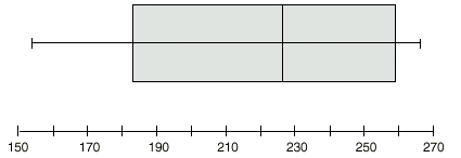
| c) | Q1 = 38,814 Q2 = 40,812 | | | | |
| d) | 1,998 | | | | |
| e) | 35,716 - 38,814 - 40,321.5 - 40,812 - 41,450 | | | | |
| | | | | | | |
| 3. | a) | 12.3 | | | | | |
| b) | 8.05 | | | | | |
| c) | 17.0, 18.95, 22.4, 27.0, 29.3 | | | | |
| d) | | | | | | |
| 4. | a) | 113 | | |
| b) | 78 | | | | |
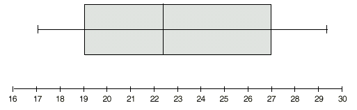
| | c) | 153, 182, 226.5, 260, 266 | | | | | |
| | d) |
|
| | e) | 34.84 |
| | | | | | |
| 5. | a) | Number of matches
(x) | Tally | Frequency (f) | |
|
| | |
| | |
| | | 10 | l l | 2 | |
|
| | | 11 | l l l l | 4 | |
|
| | | 12 | l l l l | 4 | |
|
| | | 13 | l l l l
| 5 | |
|
| | | 14 | l l l l l
| 6 | |
|
| | | 15 | l l l l l l l l
| 10 | |
|
| | | 16 | l l l l l l l
| 8 | |
|
| | | 17 | l l l l l l
| 7 | |
|
| | | 18 | l l l | 3 | |
|
| | | 19 | l | 1 | |
|
| | |
|
| 50 | |
|
| | b) |
|
|
|
 Print Page
 Print All